The Ephemerides Mechanism: A High-Precision Resonant HDC Instrument¶

"Can't stop the signal, Mal. Everything goes somewhere, and I go everywhere." — Mr. Universe, Serenity (Joss Whedon, 2005)

Signature epigraph of the spectral-research collection. The body of work — validated results and rigorous falsifications alike — was offered through conventional channels and dismissed as foolery. The math stands independently. The discipline since: ship every result, falsifications included, with full reproducibility and per-row provenance (the Mathematical Provenance Method). A corpus that publishes its own invalidations is harder to dismiss than one that doesn't, and propagates through every channel that ingests open research. The signal is in the world; it goes everywhere now.

Authors: Gemini CLI (initial scaffolding); Steven Kirkland & Claude Opus (Phase 9 ALU-native) Date: May 2026 (initial; living-document) Status: v0.29.0 (current stable on PyPI; default pip install) — production cut of the v0.29.x cycle (single rc; 0.29.0rc1 verified on TestPyPI before merge). v0.29.0 ships the channel-basis dual-path spike: opt-in es_channel_basis_method(..., ES_BASIS_METHOD_TURN_INTEGER) route that does cyclic-group-native quarter-turn decomposition (notebook §1.4: every gear is ℤ/nℤ, quarter turns are bit patterns, no × π in the global argument). The existing es_channel_basis is preserved as-is and still delegates to LEGACY → Tier 2a Python-vs-C byte-parity continues byte-for-byte; the TURN_INTEGER route is opt-in and additive. ABI v9 → v10 (additive); encoder hot path unchanged (52-body uint32 phase residues byte-identical to v0.28.1). C/Python byte-parity preserved on both routes (sibling splitmix64_phases and splitmix64_turn_integer_basis mirrors). JPL Power-of-Ten clean (pins 49 funcs / 109 asserts / density 2.22). See §4 release history below for the version-by-version landing record. The legacy v0.19.0 status banner used to attempt a chronological summary inline; that pattern didn't scale past v0.19.0 and was never updated thereafter. This banner now points at the canonical sources — python/CHANGELOG.md, ROADMAP.md, and §4 below — for current state, and gives only a brief shape-of-the-project snapshot.

Project navigation + state-pointer¶

ReadTheDocs landing — https://mlehaptics.readthedocs.io/en/latest/ — is the canonical pointer to the current state across all sister notebooks in this project.

This notebook is the active ephemerides-spectral notebook; future ephemerides framework additions land here. For sister notebooks (chess-spectral, chess-spectral-4d, antikythera-spectral, doom-spectral, othello-spectral, logo, mfo-spectral) and any new sister projects, the RTD landing is the canonical index — those notebooks are snapshots and will not be back-ported into; new framework developments are recorded here and pointed to from the RTD landing.

Brief shape-of-the-project snapshot (as of v0.26.0):

Two-stage architecture: integer-ALU phase-residue encoders (bip Python / c native / complex128 reference) feeding an FPU complex64 HD pipeline (syzygy, observer-bind, eclipse-probability). 52-body roster (v0.16.0 Tier-1 expansion). SPICE-free runtime. JPL Power-of-Ten audit baseline (all 10 rules satisfied since v0.13.9). Two-stage-architecture parity Tier 1 + Tier 2a + Tier 2b complete (v0.6.0 / v0.6.1 / v0.7.0 — every encoder-touching bridge method has a paired C path).
v0.20.x–v0.21.x — physical instruments + cross-channel couplings: Geodetic / Electromagnetic / Magnetic-Multipole / Fluid catalogs; eleven cross-channel coupling surfaces (topography ↔ gravity admittance, magnetic-derived dynamo constraints, orographic atmospheric forcing, interior-derived rotational constraints, magnetic ↔ atmosphere coupling for giants, tidal-resonance ↔ migration, atmospheric-escape ↔ magnetic shielding, heat-flow ↔ tidal heating, volcanic outgassing ↔ atmosphere, heliocentric flux ↔ surface temperature). Plus the v0.22.0 trajectory + sensing layer (ballistic, ICBM, look-angle, BC-differential).
v0.23.0 — spin-orbit resonance ↔ rotation lock catalog.
v0.24.x per-body methodology arc (the most recent extension):
action-angle decomposition — Mercury / Luna / Mars (v0.24.0 / v0.24.1 / v0.24.2; rigid-body stable / commensurate / chaotic);
continuum normal-modes — Sun (v0.24.3 helioseismic p-modes);
shape-residual on the Chandrasekhar 1969 ellipsoidal sequence — toroidal J₂ (v0.24.4);
bounded-local Laplacian for a hotspot trajectory on a body WITH plate tectonics — Hawaii hotspot chain (v0.24.5);
radiation-coupled drift for small bodies — Yarkovsky/YORP (v0.24.6);
bounded-local Laplacian for a cogenetic family on a body WITHOUT plate tectonics — Mars Tharsis (v0.24.7);
temporal quasi-periodic cycle with prediction-track-record observable — Axial Seamount (v0.24.8);
dynamical-regime classifier — eigenbasis-projection meta-consumer that treats the v0.24.0–v0.24.8 ships themselves as ground-proof rows (v0.24.9; the classifier's "training step" is np.linalg.eigh — closed-form, deterministic, byte-identical, no SGD anywhere);
OOS probe roster + classifier calibration-ratio metric — surfaces the latent diagnostic that the v0.24.9 classifier exposes through distances_to_all but doesn't summarise (v0.24.10).
Live on PyPI: pip install ephemerides-spectral.
Foundational-ontology sister-notebook (May 2026): mfo_spectral_research_notebook.md — Metric Field Ontology, one candidate foundational-ontology framing hosted in the project (cavity-instrument analogy for matter; fractal metric field; ~11D dimensional structure motivated independently from gauge-group + spectral requirements). Not the project's endorsed answer over alternatives. Cited from §20.2.1 / §20.4.0 / §20.7 as a worked example of "matter modelled as some kind of excitation" — §20 does not pick a spatial-structure side and treats the current modelling stance as provisional (FFT-untruncation framing, §20.4.0). Future MPM target.
§20 + §21 — the symmetric MPM screening sections: §20 names the producer-side screening failure (orphan-from-instrument; string-theory critique through the MPM lens); §21 names the evaluator-side screening failure (rejection-by-tool-of-creation; banning the use of a tool is the mark of a fool). Both fail for the same reason — judging by surface markers instead of by reproducible content. §21 anchors the principle on the historical precedent of the orbital-mechanics chain DE441 traces back to (Copernicus / Bruno / Galileo / Kepler — every one suppressed in their time, every one now load-bearing in the framework this project consumes); §21.3 names the disability-accommodation dimension explicitly (categorical tool bans — calculators, screen readers, voice dictation, AI assistance — function as participation barriers for contributors who depend on those tools, including those with aphantasia, ADHD, dyslexia, motor disabilities, and many other cognitive and physical variations); §21.5 documents the four-screen discipline this project applies to its own contribution gate.

Original (frozen) v0.19.0 status banner (preserved for historical context):

Living modular package. Headline state at v0.19.0: 52-body roster (v0.5.0 baseline of 38 → v0.15.0 expansion to 43 (Uranian classical + Charon) → v0.16.0 Tier-1 expansion to 52 (4 Saturnian Lagrange trojans Telesto/Calypso/Helene/Polydeuces — first L4/L5 entries in BODIES, multiplicity-2 Laplacian degeneracy at host frequency; 3 Jovian irregulars Himalia/Pasiphae/Sinope; Neptune sub-graph completion Proteus/Nereid)); SPICE-free runtime (v0.5.0); patch-shrinks-residual benchmark VINDICATED on planets (v0.5.2 — Mars 99.2 %, Mercury 99.9 %, Jupiter 97.6 %, Saturn 96.0 %) and on moons (v0.5.5 — 5 of 6 targets 93–99 %); C/Python parity Tier 1 + Tier 2a + Tier 2b complete (v0.6.0 / v0.6.1 / v0.7.0). Sol Symphony Times (v0.8.0); ITN pathway find-tubes (v0.8.1); body-identity rename Earth→Terra / Moon→Luna (v0.9.0 BREAKING); Sol Time naming overhaul (v0.9.1); CLI adaptive synonym for the breathing/Phase-9 LUT (v0.9.2). STLT (v0.10.0 — Meton's 432 BCE solstice). SPrT (v0.11.0 — gravitational + orbital-kinematic time dilation; six published validations to 0.30 %). JPL Power-of-Ten audit baseline (v0.11.2; rule-by-rule fixes v0.13.4–v0.13.9 closed every rule). Sol Kinematics (v0.12.0); Sol Dynamics (v0.13.0 — Earth-Sun force 3.54×10²² N validated to 0.01 %; virial theorem holds to 0.5 %). Pre-merge docs+parity hygiene check (v0.13.3 soft-warning workflow). Sol Moon Times complete (v0.14.0–v0.15.0 — Galileans + Saturnians + remaining 8 moons + Uranian classical + Charon binary-planet case; BODIES 38 → 43, ABI v6 → v7).

Living document. Sibling to: - ./antikythera_spectral_research_notebook.md — same-folder sibling. Where ephemerides-spectral encodes the live JPL DE441 ephemeris, antikythera-spectral encodes the cyclic-group / Laplacian-eigenbasis structure of the ca. 150–60 BCE bronze mechanism. The two projects share the spectral / cyclic-group framing and the Pyodide bridge contract; they sit side-by-side because they are related enough to share the folder, but the bronze and DE441 are separate evidentiary objects so the notebooks are not consolidated. - ./doom_spectral_research_notebook.md — same-folder sibling. Where ephemerides-spectral applies the BIP Z_{2^32} substrate + Phase-9 adaptive-coupling apparatus to the celestial N-body problem, doom-spectral applies the same substrate to the original DOOM (1993, id Tech 1) engine: BSP-tree map as a 2D Grid Laplacian (Blockmap) coarse-grained into a Sector super-graph, Z-elevation as a scalar fiber, raycasting as a dynamic sheaf Laplacian, sound propagation as heat-equation diffusion, and entity kinematics encoded directly as integer phase residues. First sibling that ports the BIP/Phase-9 machinery to a non-celestial-mechanics problem. - ../chess-maths/chess_spectral_research_notebook.md — §20.13–§20.17 explicitly aligns the chess Z_{640} phase-operator engine with this BIP design at the group-theoretic level; the cosine LUT pattern transfers between the projects. §20.21 frames doom-spectral as the fourth sibling and tabulates the Track 1 / Track 3 / Track 4 correspondences (2D Grid Laplacian; dynamic sheaf raycast; heat-equation diffusion). - ../addressing-maths/ADDRESSING_MATHS_RESEARCH_PLAN.md — the formal substrate (cyclic-group / Diophantine / packing).

0. Framing¶

The Ephemerides Mechanism (implemented in ephemerides-spectral) is the high-precision evolution of the Antikythera HDC paradigm. While the Antikythera mechanism was a masterpiece of bronze-age rational approximation, the Ephemerides Mechanism uses modern JPL ephemeris data to build a resonant HDC state vector ($D=65536$) that natively encodes celestial dynamics and their perturbations.

0.0 The Mathematical Provenance Method¶

The methodology shipped in v0.24.x and consumed by v0.24.9's regime classifier has a name we use throughout the rest of the notebook: The Mathematical Provenance Method.

The naming-discipline matters. Surface-level the v0.24.9 classifier looks like a machine-learning pipeline — labelled examples, a feature matrix, a decomposition, a nearest-neighbour query, an out-of-distribution flag. But none of the artefacts that make something machine learning are present:

Machine learning has	Mathematical Provenance Method has
Stochastic gradient descent	Closed-form `np.linalg.eigh`
Random initialisation	Deterministic eigenbasis (byte-identical on rerun)
Hyperparameter search	No knobs — the eigenbasis is a property of the data
Train / validation / test splits	All rows are ground-proof (observed physics, citable)
Loss functions	None — the eigendecomposition is a fixed-point of the data, not minimised
Pseudorandom anywhere	Nowhere
"The model" as separate artefact	The data IS the model

What we do have:

Ground-proof rows. Each entry in _research/dynamical_regime_data.py::REGIME_EXAMPLES is a real physical system whose features (timescale, spatial scale, stability, commensurability, prediction track, dimensionality, forcing class) are sourced from published literature. Adding a row is a deterministic schema extension, not a "training step."
Closed-form mathematical objects. Standardisation, covariance matrix, principal components, Mahalanobis-style distances — all closed-form algebra over the labelled rows. np.linalg.eigh is the only "computation"; it is byte-identical across reruns on the same input.
Provenance. Every row points back to a SOURCES dict entry (citation key + textual reference). When v0.24.11 added Pluto-Charon, it cited Brozovic 2015 + Stern 2015 + Showalter-Hamilton 2015. When v0.24.12 added Loki Patera, it cited Rathbun 2002 + de Kleer 2017+ + Peale-Cassen-Reynolds 1979. The eigenbasis is constructed from citable physics, not fit to observations.

The discipline implications are concrete:

Reproducibility is byte-level. A v0.24.12 install on machine A and machine B compute the same eigendecomposition to the last bit. There is no pseudorandom seed because there is no pseudorandom anywhere.
Adding a row is a schema action, not a learning action. v0.24.11's Path-B closure of v0.24.10's schema-gap explicitly chose to extend the schema (add Pluto-Charon as a ground-proof row) rather than engineer a new feature axis. The latter would change eigenbasis numerics; the former is a clean act of adding citable physics. v0.24.12 does the same, densifying the temporal-cycle regime.
Out-of-distribution flagging is honest. When the v0.24.10 OOS probe roster shows Vesta with calibration_ratio = 0.98, that's the eigenbasis saying "I have no close neighbour — I genuinely don't know." When v0.24.12 added Loki and Vesta's calibration ratio dropped to ~0.79, that's the same eigenbasis saying "I now have a close-spatial-scale neighbour, but my regime label rigid_body_chaotic_obliquity is the WRONG physics" — pinned in tests as a v0.24.12-introduced schema-gap, surfacing the next ship's target.
The classifier is its own provenance trail. Every classification decision can be traced back to specific ground-proof rows + specific citations. There is no "model said so" — there is only "the eigenbasis projection of these specific labelled examples (citations attached) places this probe nearest to row X."

Where machine learning bills itself as "extract patterns we don't already know from data we don't fully understand," the Mathematical Provenance Method bills itself as "project labelled physics through a closed-form eigenbasis and ride the consequences." The discipline says: when the answer needs to be defensible, prefer the method whose every step has citable mathematical provenance.

This naming is now used downstream. v0.24.x ships are Mathematical Provenance Method ships; v0.24.x catalog rows are ground-proof rows, never "training data."

0.1 From Gears to Fibers¶

The Antikythera mechanism used coprime gear ratios to encode mean motion. In the Ephemeris Mechanism, these unperturbed orbits form the diagonal content of our system Laplacian. The real "innovation" of this project is the treatment of gravitational perturbations as off-diagonal fiber couplings.

Just as a chess capture redistributes field energy across piece-specific movement graphs, the mass of Jupiter dynamically "captures" or perturbs the phase of Mars. In our HDC encoding, these interactions are modeled as interaction hypervectors that fire based on body proximity and resonance, allowing the N-body problem to be computed through vector superposition and correlation.

1. Mathematical Architecture¶

1.1 Encoding Primitives¶

Unitary Binding: We use circular complex bases (magnitude 1 per component) to ensure that all binding operations (observer shifts, temporal advances) are unitary rotations that preserve the total energy (Norm=1.0) of the hypervector.
Coprime Roll Binding: Mirroring the chess-spectral (67, 7) pattern, we use coprime cyclic rolls to bind geographic coordinates (lat/lon) to the global system state.

1.2 Observer-Agnosticism¶

The system state $H_{sys}$ is barycentric. A topocentric "Local View" $V_{local}$ is extracted by binding a unitary Observer Operator $O$: $$V_{local} = H_{sys} \otimes O(Body, \lambda, \phi)$$ This allows for instantaneous state extraction from any position on any supported celestial body.

1.3 Syzygy as a Spectral Event¶

Eclipses and conjunctions are not "searched" in the traditional sense; they are detected as alignment peaks with a pre-calculated Syzygy Operator $S$: $$P_{syzygy} = \langle H_{sys}, S \rangle$$ This treats high-precision astronomical events as primary spectral signatures within the HDC space.

1.4 Mathematical positioning of the "breathing Laplacian"¶

The Phase-9 phrase "breathing Laplacian" is a project codename. This subsection names the formal mathematical objects so a reader from spectral graph theory, dynamical systems, or solid-state physics can place the construction in the literature their discipline already proves theorems about.

The static piece. The Phase-8 Laplacian is a Hermitian matrix on the body-interaction graph $G = (V, E)$ with $|V| = 26$ bodies:

\[L_{\text{LTI}} = L_{\text{trunk}} + L_{\text{PN}} + L_{\text{static}}\]

where $L_{\text{trunk}}$ is the diagonal of mean motions $\omega_i = 2\pi / P_i$, $L_{\text{PN}}$ is the Mercury post-Newtonian correction, and $L_{\text{static}}$ is the symmetric off-diagonal of gravitational fiber weights. Evolution is the Schrödinger-like flow $\psi(t) = e^{-i L_{\text{LTI}} t} \psi(0)$ on the cyclic-group manifold.

The dynamic piece. Phase 9 promotes the off-diagonal weights to functions of the current phase state:

\[W_{ij}(\phi) = W_{ij}^{(0)} \cdot \bigl(1 + \alpha \cos(n_{ij} \phi_i - m_{ij} \phi_j)\bigr)\]

so the Laplacian itself becomes state-dependent: $L = L(\phi(t))$. The flow is no longer a single matrix exponential — it is integrated chunk-wise in 30-day steps with $L$ recomputed each chunk.

What this is, in three vocabularies.

Spectral graph theory / linear algebra. A state-dependent (non-autonomous) graph Laplacian. The instantaneous spectrum of $L(\phi(t))$ defines the system's normal modes at each instant; the dynamics evolves through these modes as $\phi$ re-organises. This is the "vibrating-lattice" intuition formalised — at every instant we have a bona-fide lattice with bona-fide phonon-like modes; what changes is the Hamiltonian itself.
Dynamical systems / synchronisation theory. An adaptive Kuramoto-family network with phase-difference-dependent (PDDP) coupling. Standard Kuramoto fixes $K_{ij}$ and varies $\phi$; we vary both, with $K_{ij}$ a smooth function of $(\phi_i, \phi_j)$. The literature calls this adaptive coupling or plastic coupling, with a substantial body of synchronisation-resilience results we can lean on (Berner et al. on adaptive phase oscillators; Sakaguchi-style PDDP rules).
Physics framing. A resonance-modulated coupling of phase oscillators, structurally analogous to the Discrete Nonlinear Schrödinger / Gross-Pitaevskii equation on a graph in the limit where amplitudes are pinned to unit norm and only phases evolve. The coupling kernel $\cos(n\phi_i - m\phi_j)$ is the standard $n{:}m$-resonance lobe; that we model the J–S 5:2 with $\alpha = 0.1$ is a phenomenological choice, not derived from a Lagrangian. A first-principles derivation would route through Hamilton's equations on the Delaunay variables — out of scope for v0.1.0; flagged as future work.
Discrete differential geometry / curvature in motion. The cleanest single-phrase reading is state-dependent discrete Ricci curvature — the breathing Laplacian is curvature in motion. A weighted graph carries a discrete analog of Ricci curvature (Forman-Ricci $\mathrm{Ric}_F$, Ollivier-Ricci $\kappa_{OR}$, or Bakry-Émery's $\Gamma_2$ / curvature-dimension condition $\mathrm{CD}(\kappa, \infty)$); each is a function of the edge weights $W_{ij}$ and the edge-incidence pattern. When edge weights are state-dependent — $W_{ij}(\phi) = W_{ij}^{(0)}(1 + \alpha \cos(n_a\phi_a - m_b\phi_b))$ — the discrete Ricci curvature on each resonance edge becomes a periodic function of the phase state. The spectral identity is the Bochner-Lichnerowicz analog: the Laplacian's spectrum is bounded below by curvature via $\lambda_2 \geq \kappa$ (CD($\kappa$, $\infty$) on a graph yields the same eigenvalue gap inequality as on a Riemannian manifold). What "breathes" in our codename is exactly this curvature: it inhales and exhales over the resonant-phase angle, and the spectral gap $\lambda_2$ tracks it.

This reading also names the v0.5.x roadmap target precisely. The static $L_{\text{trunk}} + L_{\text{PN}} + L_{\text{static}}$ piece sets a fixed baseline curvature — the encoder's "metric." The Phase-9 modulation adds a curvature flow that is forced, not relaxed: where Hamilton-style discrete Ricci flow would evolve the metric to flatten the curvature toward a smooth limit, our case is the opposite — the curvature is forced to oscillate by the phase-coupling rule. It is "phase-locked Ricci flow" — the geometry doesn't relax but pulses with the natural resonance frequencies of the bronze antikythera's gear ratios. The diagnosed-fiber overlay (§8) and the LS-fit catalog (§9) are then empirical curvature corrections: each catalog patch adds a periodic delta to one body's residual that, in the curvature reading, nudges the local Ricci curvature on the patched edge into agreement with what the actual ephemeris demands.

Why "breathing" is metaphor, not vocabulary. The codename captures the rhythm — coupling strengths inhale and exhale with the resonant-phase angle — but it does not connect to the literature's existing theorems. State-dependent graph Laplacian is the name to grep for in spectral-graph papers; adaptive Kuramoto network is the name to grep for in synchronisation papers; state-dependent discrete Ricci curvature (or "curvature in motion") is the name to grep for in discrete differential geometry / Bakry-Émery / Ollivier–Ricci papers; parametric coupling — and its synonyms parametric oscillator network, parametric resonance, parametric instability, and the Mathieu / Hill non-autonomous oscillator family — is the name to grep for in classical-mechanics, accelerator-physics, and nonlinear-dynamics papers. The substance is the same: a coupling strength that is itself a periodic function of time (here driven by the phase angle $n_a\phi_a - m_b\phi_b$, equivalent under our 1^st-order phase rotation to a slow time variable). Faraday (1831, surface-wave parametric instability) opens the field; the Mathieu equation $\ddot x + (\delta + \varepsilon \cos t)\,x = 0$ supplies the canonical stability / instability tongue diagrams (the Strutt diagram), and the modern accelerator-physics machinery on synchro-betatron coupling + dispersion-driven parametric resonance carries the small-α perturbative regime our $\alpha = 0.1$ Phase-9 modulation lives in. Vibrating lattice captures the right intuition (phonon-like instantaneous spectrum) but is a 2^nd-order Newtonian framing, whereas our flow is 1^st-order phase rotation. We use "breathing" in headings and section labels for project continuity, and the precise vocabulary in prose so future readers can find their way out of our codename and into the canonical literature — depending on which of the four formalisms (state-dependent Laplacian / adaptive Kuramoto / Ricci-in-motion / parametric coupling) maps best to the theorem they need.

What about a true vibrating-lattice formulation? The Phase-8 propagator $e^{-iLt}$ on the cyclic-group manifold is isomorphic to the linear-phonon propagator on a 1D ring lattice in the eigenmode basis: each mode rotates at its eigenvalue. The Phase-9 modification then plays the role of phonon–phonon scattering (anharmonic coupling). If we ever want to study energy transfer between modes — Fermi-Pasta-Ulam-Tsingou-style equipartition, soliton-on-a-ring, etc. — that is the framing to import. v0.1.0 stops short of any nonlinear-mode bookkeeping; we evolve in the body-index basis, not the eigenmode basis.

2. Implementation & Validation¶

2.1 The ephemerides-spectral Package¶

The project is scaffolded as a standalone PyPI-ready package with: - bridge.py: Pyodide-JSON contract for web frontend integration. - _research/: Deterministic snapshots of the core instrument logic. - codegen/: Automatic manifest and data freezing infrastructure.

2.2 Results¶

The prototype successfully: - Extracts true ecliptic longitude from JPL kernels. - Maintains hypervector integrity (Norm=1.0) through frame shifts. - Detects proximity-based gravitational interaction terms. - RBS-HDC Advancement: Verified a 305× speedup using FPU-less integer arithmetic. - Structural Limit Identified: Confirmed a ~0.0002 rad error floor (Phase 8) due to the static LTI Laplacian assumption and Newtonian mean-motion constraints. - Phase 9 Breathing Couplings: Replaced the static off-diagonal weights with phase-dependent modulation via an integer cosine LUT (1024 × int32, Q1.14). The Jupiter–Saturn 5:2 resonance term is now implemented end-to-end without leaving the integer ALU. - Fixed-Point Discipline: All angular frequencies are stored as signed int64 in residues/day (Q-format with MODULO = 2^32 residues per revolution); the Q-format underflow guard, pre-flight bounds check, and scoped overflow trap are documented in resonant_bit_serialized_hdc_evaluation.md §8.3–§8.4. - Cross-pollination: chess-spectral §20.13–§20.17 explicitly aligns the chess Z_{640} phase-operator engine with this BIP design at the group-theoretic level; the cosine LUT pattern transfers between the projects (chess pays an explicit % 640 per op, ephemerides gets cyclic-group reduction free as uint32 overflow).

3. Future Tracks¶

Shipped since this section was first written¶

Download DE441: Scale the validation suite to the full 3.3 GB JPL kernel. — shipped v0.3.0. Full ±14,000 yr sweep against DE441 ground truth (figures/de441_full_sweep.md).
Phase 9 Coverage: Extend breathing couplings beyond the J–S 5:2 term. — shipped v0.2.0 (Neptune–Pluto 3:2 + Io–Europa 2:1 + Europa–Ganymede 2:1) and v0.5.0 (Mimas–Tethys 4:2 Cassini Division + Enceladus–Dione 2:1 + Titan–Hyperion 4:3). Seven resonance entries total.
~~Spectral syzygy window search.~~ — shipped v0.3.1 as bridge.find_syzygies + CLI find-syzygies. ~1000× faster than the v0.3.0 point-evaluation eclipse --jd for window queries; uses the natural cyclic-group decomposition (synodic + draconic month + Saros) to enumerate candidates in closed form.
~~DE441 error-spectrum FFT diagnostic.~~ — shipped v0.3.1 as research/de441_error_spectrum.py. Per-body FFT of the DE441-truth residual identifies smoking-gun missing-coupling signals; surfaced the Jupiter–Saturn 9.56 yr ±45° peak that motivates the diagnosed-fiber catalog.
~~Native C backend.~~ — shipped v0.3.1 (cibuildwheel platform wheels, backend="c", ~1000× speedup vs Python BIP, byte-exact parity).
~~Diagnosed-fiber runtime overlay (Python side).~~ — shipped v0.4.0. See §8 below for the architecture.
~~C-side overlay (ABI v2).~~ — shipped v0.4.1. Native backend now applies the overlay; cross-backend byte-exact parity with patches active.
~~SPICE-free runtime.~~ — shipped v0.5.0. Codegen bakes initial phases into _data/initial_phases.json; pip install works out of the box.
~~Patch-shrinks-residual benchmark.~~ — shipped v0.5.1 (PARTIAL) → v0.5.2 (VINDICATED). See §9 below for the methodology + result.

Still to come¶

First-Principles Phase-9 Derivation: v0.1.0's $\alpha = 0.1$ J–S breathing depth is phenomenological. Deriving the modulation depth from a Hamilton/Delaunay-variable Lagrangian (with Lie-series perturbation theory around the 5:2 resonance) would replace the placeholder with a first-principles value. Connects to the adaptive-Kuramoto literature on derived-from-physics PDDP rules (cf. §1.4). v0.5.2's LS-fit catalog (§9) is the empirical analog — Fourier-correction patches that first-principles α should ultimately make redundant for the bodies inside the resonance set.
DE441 vs DE442 spectral error signature (research experiment): build two BIP instruments calibrated separately from DE441 and DE442; encode the same JD on both; project per-body residue deltas onto the Laplacian eigenbasis. Hypothesis: DE442's corrections to DE441 occupy a coherent eigenmode subspace — the spectral signature of the kernel update. If we can find a correlate, we can predict where ephemeris error correction is structurally needed without having the corrected kernel in hand. The natural-coprime decomposition from §6 would be the basis for that prediction.
Multi-Millennium Sweep against breathing couplings active: Re-derive the historical anchors for the Metonic and Saros cycles against the full DE441 sweep (already done at the planet level; multi-millennium re-derivation with the v0.5.x resonance-corrected encoder is the follow-up).
CORDIC Topocentric Rendering: The cosine LUT is the first half of a CORDIC observer-binding pipeline; the rotation half can subsume the topocentric lat/lon bind.
Resonant Bit-Serialized Hardware: Port the BIP integer-only evolution to bit-serial hardware simulations (Verilog/SystemC). The cosine LUT becomes block RAM; the omega * step multiply becomes a fixed-precision multiplier.
~~Moon residual root-cause investigation (v0.5.x)~~: shipped v0.5.3 → v0.5.5 as the three-phase moon programme. Phase A (diagnostic) ruled out the frame-mismatch hypothesis. Phase B (v0.5.3) fixed period truncation; 13 of 17 moons dropped 30-1450× in RMS. Phase C (v0.5.5) authored 5 LS-fit catalog patches at 93-99% shrinkage. Four moons remain physics-specific follow-ups (metis / thebe / rhea / phoebe).
~~C/Python parity Tier 1~~ (v0.6.0): shipped. find_syzygies + get_breathing_modulation now have C twins; ABI v3. The tests/test_parity_smoke.py PARITY_TARGETS table is the durable SSOT for what's at parity vs what's pending.
C/Python parity Tier 2 (v0.7.0): get_local_view and get_eclipse_probability still operate on the FPU complex128 hyperdimensional state. Lifting the C runtime to carry HD state via channel-basis emission at codegen time is the architectural change; the parity smoke test's two tier2_skip entries flip to parity when this lands.
LTC (Lunar Coordinated Time) (v0.6.x or later): Pending NASA + international space-agency standardisation (target 2026–2028 per April 2024 White House directive). LTE440 (Lin et al. 2025) ships the underlying SPICE-format conversion ephemeris with 0.15 ns accuracy through 2050; ephemerides-spectral gains an LTC namespace in the bridge mirroring MarsTime once the LTC epoch + day-length convention are formalised.
Multi-component or coupled-T-H Hyperion patch (v0.6.x): Hyperion's chaotic rotation produces multi-peak quasiperiodic residual that single-sinusoid LS-fit hits at 75.2% (vs the 80% catalog gate). Two paths: (1) multi-component patch — one entry expressed as a list of (period, amplitude, phase) sinusoids; the v0.5.2 multi-bin idea revived for chaos rather than bin leakage. (2) coupled titan-hyperion-4to3-coupled-v2 patch — v0.5.0 wired the resonance into RESONANCES but never calibrated the coupling strength; same v0.5.2 J-S template, different bodies.

4. Release History¶

v0.29.0 — 2026-05-15. Production cut after the v0.29.0 rc cycle — channel-basis dual-path spike (TURN_INTEGER, cyclic-group-native; ABI v9 → v10 additive). Version-only bump from 0.29.0rc1 → 0.29.0 after the single-rc TestPyPI verification cycle. Cumulative content from rc1: opt-in es_channel_basis_method(seed, out, D, ES_BASIS_METHOD_TURN_INTEGER) entry point + es_basis_method_t enum that gives callers a cyclic-group-native channel-basis construction route — integer quarter-turn decomposition on the splitmix64-derived phase residue (phase = (uint32_t)(u >> 32) in Z_{2^32}; quadrant = phase >> 30; within = phase & 0x3FFFFFFF); bit-exact dispatch to (±1, 0) / (0, ±1) when within == 0; libm cos/sin only on the within-quadrant fraction (small argument, no internal reduction needed); i^quadrant rotation by pure sign/swap. Bit-exact quarter turns on every toolchain — no libm cospi/sinpi dependency, no platform feature gate, no × π in the global argument. The existing es_channel_basis is preserved as-is — delegates to LEGACY — so the Tier 2a Python-vs-C byte-parity test continues to hold byte-for-byte. C/Python byte-parity preserved on both routes: _research/portable_prng.py carries splitmix64_turn_integer_basis_element + splitmix64_turn_integer_basis (Python mirror of the C TURN_INTEGER route); sibling discipline to the LEGACY route's existing splitmix64_phases + numpy.exp(1j · φ) mirror. JPL Power-of-Ten clean (pins 49 funcs / 109 asserts / density 2.22). Mid-rc design pivot preserved in the rc1 branch history: an initial draft of this spike (commit 1b860f8) used C23 / Apple-libsystem cospi/sinpi to bypass the × π rounding loss but introduced a platform-feature-detection problem; the mid-rc design discussion concluded the phase is already a rational fraction in Z_{2^32} and cospi was a half-measure delegating quarter-turn-aware-reduction to libm when the integer cyclic-group representation does it exactly. The TURN_INTEGER pivot replaces the cospi route + the CMake check_function_exists(cospi) feature detection; captures the same precision benefit using only universally-available primitives. Verified on TestPyPI before the production cut: 0.29.0rc1 boots cleanly in an external venv on Python 3.10-3.14; plugin-tier Profile.native resolves with ABI v10; LEGACY method byte-identical to default es_channel_basis; C/Python TURN_INTEGER byte-parity holds on the live wheel; encoder hot path produces 52 uint32 residues at J2000. The cibuildwheel matrix (Linux/macOS-14/Windows × py3.10-3.14, 18 jobs) all green. No code change from v0.29.0rc1; no ABI change (ES_ABI_VERSION = 10 unchanged from rc1); encoder hot path is unchanged (52-body uint32 phase residues byte-identical to v0.28.1). Future float64 path: when a future cycle ships a complex128 HD-state, the within-quadrant × (π/2 / 2^30) multiply's 1 ULP double-precision rounding loss becomes visible above the float32 cast → Cody-Waite hi/lo splitting of the π/2 constant becomes the right next move at that point. Out of scope for v0.29.0 whose output is complex64.
v0.29.0rc1 — 2026-05-15. Channel-basis dual-path spike (cyclic-group-native quarter-turn decomposition; ABI v9 → v10 additive). First rc of the v0.29.x cycle is a small precision spike that honours the notebook §1.4 framing: every gear is a faithful representation of ℤ/nℤ; quarter turns are bit patterns; π should not appear in the global argument when integer arithmetic is already exact on the cyclic-group level. The shipped LEGACY route does phi = (u >> 11) · (2π / 2^53) as a software multiply then calls libm cos/sin on the radian result — composing two argument-reductions and leaving ~2 ULP of error at quarter-turn channels. The new TURN_INTEGER route works in turns from the start: phase = (uint32_t)(u >> 32) is the cyclic-group element in Z_{2^32}; quadrant = phase >> 30 and within = phase & 0x3FFFFFFF is the integer quarter-turn decomposition; when within == 0 the route dispatches bit-exact (±1, 0) / (0, ±1) from i^quadrant; otherwise it computes cos(a) / sin(a) for a = (double)within · (π/2 / 2^30) ∈ [0, π/2) and applies the i^quadrant rotation by pure sign/swap (no float math). Quarter-turn channels are bit-exact by construction on every toolchain — no libm cospi/sinpi dependency, no platform feature gate, no × π in the global argument; only universally-available libm cos/sin + integer arithmetic. New C surface: es_basis_method_t enum (ES_BASIS_METHOD_LEGACY = 0, ES_BASIS_METHOD_TURN_INTEGER = 1) + es_channel_basis_method(seed, out, D, method) entry point. The existing es_channel_basis is preserved as-is — delegates to _method(..., LEGACY) — so the Tier 2a Python-vs-C byte-parity test continues to hold byte-for-byte; the TURN_INTEGER route is opt-in. Why not flip the default in this rc? The byte-parity test pins numpy.exp(1j · φ) against the C output; numpy uses × 2π in software too, so TURN_INTEGER bytes differ from Python's. Flipping would break parity. The dual-path is "bench-first; decide later": new scripts/bench_turn_integer_basis.py (NDJSON output, one record per line per project convention) sweeps (seed, D) points + a representative HDC roll-and-accumulate, reporting per-element drift / unit-magnitude error / accumulator-norm delta / count of quarter-turn bit-exact dispatches. Quantitative findings inform whether to graduate TURN_INTEGER to default + update the Python mirror in a future cycle, or keep LEGACY as the default and TURN_INTEGER as the precision-on-demand route. Design pivot mid-rc: an initial draft of this spike used C23 / Apple-libsystem cospi/sinpi (commit 1b860f8 on the feature branch); the design discussion that followed concluded that the phase is already a rational fraction (Z_{2^32}) and cospi was a half-measure delegating quarter-turn-aware-reduction to libm when our own integer representation does it exactly. The TURN_INTEGER pivot replaces the cospi/sinpi route and the CMake check_function_exists(cospi) feature detection; it captures the same precision benefit using only universally-available primitives. Future float64 path: when a future cycle ships a complex128 HD-state path, the within-quadrant × (π/2 / 2^30) multiply's 1 ULP double-precision rounding loss becomes visible above the float32 cast — Cody-Waite hi/lo splitting of the π/2 constant becomes the right next move at that point. Out of scope for v0.29.0rc1 whose output is complex64. JPL Power-of-Ten clean: pins ratcheted 46 → 49 functions / 102 → 109 assertions (density 2.22, well above the ≥ 2.0 floor); no goto; no malloc; all loops bounded; every new function ≥ 2 asserts. Python wiring: EXPECTED_ABI_VERSION 9 → 10; new helpers native_channel_basis_method + native_channel_basis_turn_integer; new constants ES_BASIS_METHOD_LEGACY / ES_BASIS_METHOD_TURN_INTEGER; __all__ updated. srmech profile descriptor [profile.native].expected_abi_version 9 → 10. New tests/test_channel_basis_dual_path.py pins six invariants: LEGACY-method route byte-identical to default es_channel_basis across the existing Tier 2a parity grid; TURN_INTEGER shape/dtype/unit-magnitude; quarter-turn dispatch structurally bit-exact (any near-quadrant element has its orthogonal component exactly 0.0f); soft ratchet (TURN_INTEGER ≤ LEGACY on |mag - 1| plus a ~6e-8 fairness allowance); invalid enum rejected via ES_ERR_INVALID_KIND; deterministic across calls. C/Python byte-parity preserved on both routes: _research/portable_prng.py gains splitmix64_turn_integer_basis_element + splitmix64_turn_integer_basis (Python mirror of the C TURN_INTEGER route); tests/test_channel_basis_parity.py extends the existing LEGACY parity battery with sibling test_channel_basis_turn_integer_byte_identical_py_vs_c (same seed/D grid) + a structural quarter-turn-dispatch-bit-exact test on the Python helper. Cross-platform verified: Windows MSVC and WSL2 glibc 2.35 produce byte-identical TURN_INTEGER bytes on both Python and C sides (run with python -m pytest python/tests/test_channel_basis_parity.py to reproduce). No encoder hot-path changes — the 52-body uint32 phase residues emitted by es_encode_state / bridge.encode_state are byte-identical to v0.28.1.
v0.28.0rc5 — 2026-05-14. Phase 10a EOC C-side completion (ABI v8 → v9). Final rc in the v0.28.x stack. Closes the rc1 backend_caveat: per-body equation-of-center patches now produce byte-identical phase residues on both backend="bip" AND backend="c" across all 52 bodies at every Δt tested. C-side: new patch kind ES_PATCH_KIND_ECCENTRICITY_CORRECTION = 2; es_patch_t extended with 3 trailing double fields (eccentricity, mean_anomaly_at_j2000_rad, n_rad_per_day); Newton-Kepler evaluator es_eval_eoc_residue in c/src/es_patches.c — bounded 30-iter Newton on E − e·sin(E) = M (tol 1e-14 rad, warm-start E = M + e·sin(M) for e > 0.6); half-angle true-anomaly ν = 2·atan2(√(1+e)·sin(E/2), √(1−e)·cos(E/2)); principal-branch wrap via floor-based modulo (single libm call; no unbounded while-loop). Returns (ν(t) − M(t)) − (ν(J2000) − M_0) mapped to uint32 residue — same anchoring as the Python reference, byte-for-byte mirror. New es_clear_eoc_patches selective clear by kind. JPL Power-of-Ten clean: every new function carries ≥2 asserts (Rule 5); no goto (Rule 1); no malloc (Rule 3); all loops bounded (Rule 2 — Newton at 30 iters; clear at ES_MAX_PATCHES = 32); each function ≤60 lines (Rule 4). Python wiring: EXPECTED_ABI_VERSION 8 → 9; EsPatch ctypes struct extended in lockstep with the C struct's trailing fields; new helpers native_apply_eoc_patch + native_clear_eoc_patches; _mirror_patch_to_native gains an EccentricityCorrectionPatch dispatch branch (bridge surfaces that go through it pick up C-side support transparently); bridge.apply_eoc_patches iterates registered patches and calls _mirror_patch_to_native, rolling back BOTH registries on any C-side rejection so the two registries never drift; bridge.clear_eoc_patches mirrors selective clear via native_clear_eoc_patches. Return envelopes gain n_registered_c_side, backends_active (e.g. ["bip", "c"] on native installs), cleared_c_side. srmech profile descriptor [profile.native].expected_abi_version 8 → 9 — srmech's loader catches v8/v9 mismatches at activation. Test ratchet flips: rc1 test_eoc_patch_is_python_only_kind → rc5 test_eoc_patch_kind_now_c_native (positive ratchet — _mirror_patch_to_native returns None on native installs). New test_eoc_patch_byte_parity_across_backends pins byte-exact EOC parity at four Δt epochs (J2000, ±1 yr, +20 yr, -100 yr); skipped cleanly on pure-Python installs. JPL audit pins updated (PIN_RULE_5_TOTAL_FUNCS 42 → 46; PIN_RULE_5_ASSERTIONS 88 → 102; density 102/46 = 2.22, well above the ≥2.0 average floor). ABI wire-format change: sizeof(es_patch_t) increased by 24 bytes (3 trailing doubles). The ABI handshake (srmech _maybe_load_native + _native_bip direct check) catches v8/v9 mismatches and degrades to pure-Python rather than producing silent garbage. After rc5 verifies on TestPyPI + autonomous merges, the v0.28.0 production-cut PR opens for human-in-loop review.
v0.28.0rc4 — 2026-05-14. Task #212 PR-c — bridge call-site migration through srmech.profile("ephemerides").native. Final PR of Task #212 (ADR-0001 §7 Step 2 call-site-migration portion). New _load_via_srmech_profile() in _native_bip.py lazily imports srmech, calls srmech.profile("ephemerides"), and reuses the loaded CDLL handle when available; the existing direct ctypes.CDLL() path remains as the fallback for sdist / pure-Python / srmech-absent environments. _native_bip.LIB and srmech.profile("ephemerides").native are now the same Python object (Python is identity, not just equality) — patch-registry runtime state stays consistent across both surfaces. Without this migration, two separate dlopen() calls of the same library file would yield two CDLL instances with independent patch-registry views (a real footgun the migration eliminates). New module global LOAD_SOURCE ∈ {"srmech_profile", "direct_ctypes", None} surfaces which path was chosen. 3 new ratchets in test_native_parity.py pin a four-way parity property: Python BIP encoder ↔ profile-loaded native ↔ direct-ctypes native (fresh CDLL on the library file) ↔ bridge backend="c" all produce byte-identical phase residues at every JD. Pure-Python additive; no ABI bump (PR-c rearranges how the library handle is obtained; no C-side surface change).
v0.28.0rc3 — 2026-05-14. Task #212 PR-b — srmech [profile.native] plugin tier + ABI v6→v8 realignment + native-parity drift fix. ephemerides-spectral's srmech profile graduates from "simple" (PR-a, v0.27.0) to "plugin" tier. New [profile.native] block in srmech_profile.toml: library = "ephemerides_spectral", install_path = "ephemerides_spectral/_native", abi_version_function = "es_abi_version", expected_abi_version = 8; 8 declared [profile.native.symbols.*] covering encoder hot path + introspection accessors. srmech's Profile._maybe_load_native() now resolves the platform-specific shared library, performs the es_abi_version() handshake, and exposes a bound ctypes.CDLL as Profile.native. Silent-rejection bug fix: _native_bip.EXPECTED_ABI_VERSION was left at 6 while the C library's ES_ABI_VERSION advanced to 8 in v0.16.0 (Tier-1 BODIES expansion, commit f1d4b82). Every wheel install since v0.16.0 silently fell back to the pure-Python BIP encoder because the ctypes shim's ABI handshake rejected the bundled library. Bumping to 8 realigns the shim with the shipped library; native acceleration is restored across the install base. Native-parity drift fix: the realignment unmasked a latent drift between c/src/es_laplacian.c and _data/initial_phases.json on 15 Mars + Saturnian moons (the bodies that depend on auxiliary mar099s + sat441 JPL kernels; both sides had been regenerated under different kernel availability). Re-running c/codegen/emit_c_tables.py against the same stub-fallback state the JSON uses makes both sides byte-agree on all 52 bodies. (rc2 was a failed-publish tombstone — the cibuildwheel Linux matrix surfaced the parity drift; rc3 absorbed the fix.) 13 new ratchets in test_srmech_profile.py (9 static descriptor checks + 4 activation-path tests; the static set pins expected_abi_version agreement with _native_bip.EXPECTED_ABI_VERSION as the single anti-drift ratchet for the silent-rejection bug class). Pure-Python additive; no ABI bump (C-side ES_ABI_VERSION stays at v8; the Python-side realignment is a catch-up only).
v0.27.0 — 2026-05-14. Production cut: Task #212 PR-a — srmech profile pattern (ADR-0001 §7 Step 2 simple-tier portion). Already shipped to production PyPI; verified via the rc1 TestPyPI cycle. Simple-tier ship — [profile.bridge] + [profile.smoke_test] + [profile.tool_schema]; no plugin-tier wiring yet (that lands in v0.28.x rc3/rc4/rc5). Mirrors the chess-spectral v1.19.0 ship. Dependency floor srmech>=0.3.1,<0.4.
v0.28.0rc1 — 2026-05-14. Phase 10a — Per-body equation-of-center catalog (PEP 440 alpha pre-release of v0.27.0). Closed-form Kepler-series patches for every non-Sun body in the 52-body BIP roster (51 patches; Sun has e ≡ 0 → no EOC contribution). New EccentricityCorrectionPatch patch kind in diagnosed_fibers.py — Newton iteration on Kepler's equation E − e·sin E = M (bounded 30-iter loop, tol 1e-14 rad) + half-angle true-anomaly formula ν = 2·atan2(√(1+e)·sin(E/2), √(1−e)·cos(E/2)). J2000-anchored by construction — patch evaluates to exactly 0 at the BIP calibration epoch (because BIP's initial_phases[i] = L_true(J2000) from DE441, not L_mean(J2000)); the patch adds (ν(t) − M(t)) − (ν(J2000) − M(J2000)) so the J2000 EOC value isn't double-counted. Exact at any eccentricity from Triton's e ≈ 1.6×10⁻⁵ through Nereid's e = 0.7507; no power-series truncation. New _research/secular_elements_data.py — 51-row J2000 Keplerian mean-elements catalog, frame partition 13 heliocentric (9 planets + 4 main-belt asteroids) + 38 parent-centric (1 Luna + 2 Mars moons + 11 Jovian + 15 Saturnian + 5 Uranian + 3 Neptunian + 1 Charon), with 16 subsystem-authority sources (Standish 1992 + Park 2021 DE441 for the planets; Chapront-Touzé & Chapront 1991 ELP2000 for Luna; Lainey 2007 MAR063 for Mars moons; Lieske 1998 E5 for the Galileans; Cooper 2006 for Jovian inner regulars; Jacobson 2000 JUP100 for Jovian irregulars; Vienne & Duriez 1995 TASS / Jacobson 2006 SAT375 for Saturnian classical; Spitale 2006 for Saturn co-orbitals + trojans; Jacobson 1998 for Phoebe; Laskar-Jacobson 1987 GUST86 for Uranian; Jacobson 2009 NEP078 for Neptunian; Brozovic 2015 for Charon; JPL Small-Body Database for asteroids). New _research/eoc_catalog.py generator — EOC_CATALOG dict (51 patches), build_eoc_patch(body), frame / parent / body selectors. New AMSC source secular_elements (literature_curated adapter): descriptor.toml + row.schema.json (draft 2020-12; 14-field row contract) + row.ndjson (51 data rows; per-row source_doi follows the v0.27.0-phase-A convention — real Crossref DOIs preferred, nodoi: for pre-Crossref JPL technical documents, isbn: for textbooks, url: for JPL SBDB); n_sources 19 → 20, adapter_class="curated" 16 → 17. Six new bridge surfaces: list_secular_elements(frame, parent), get_secular_elements(body), list_eoc_patches(frame, parent), get_eoc_patch(body), apply_eoc_patches(bodies, frame, parent), clear_eoc_patches(). Six new CLI subcommands mirror them 1:1. The LLM tool-schema export (v0.26.1 feature) auto-discovers all 6 — tool count 240 → 246, no manual schema authoring. Validation (the closed-form-algebra payoff) — 100-yr Earth-Mars syzygy sweep on v0.26.1 against textbook Mars-opposition dates collapses from 19.79 d RMS (35.32 d max) to 1.12 d RMS (3.05 d max) with terra + mars EOC patches active (94% collapse on anchor-date offsets). The closed-form Kepler-truth Δλ at BIP-opposition JDs collapses from 9.26° RMS (15.75° peak) to 0.014° RMS (0.015° peak) — a 99.85% collapse to numerical precision. The residual 1.12 d anchor RMS is the genuine off-diagonal Mars-Jupiter direct gravitational coupling, Phase 10b's target. Sun-from-SSB wobble falsified as bin-5 (20.07 yr) explanation — hypothesis tested closed-form by direct Sun-from-SSB subtraction, collapsed only 0.7% (most likely DFT side-lobe leakage from the dominant Earth+Mars EOC peak at bin 6; predicted leakage 3.0% vs observed 3.5%). Stashed at docs/srmech/notes/sun-wobble-falsification-2026-05-14.md as the first published-internal falsification of a candidate Phase-10b coupling — the MPM discipline working at the negative-result level. Backend caveat: EOC patches are Python-BIP-backend-only in v0.28.0rc1; C-side support requires an ABI bump (new ES_PATCH_KIND_ECCENTRICITY_CORRECTION) queued for v0.27.0 / v0.28.0. With EOC patches active, backend="c" returns the unpatched residue. Tests: 39 ratchets in tests/test_eoc_catalog.py — coverage (51-body, frame partition, 16 sources), period agreement vs BODIES SSOT (max rel_err 4.6e-4 Saturn), Newton-Kepler correctness vs independent closed-form (parametrized 8-body sweep), J2000-anchoring, frame discipline, AMSC dual-author parity (byte-for-byte field check + provenance completeness + source_doi prefix convention), bridge filter semantics, apply/clear round trip, Python-BIP-only kind ratchet. Plus tests/test_attested_collector.py n_sources bumps 19 → 20 and 16 → 17. Workflow regex extension in .github/workflows/ephemerides-spectral-publish.yml: tag-version regex extended from (\d+\.\d+\.\d+(?:rc\d+)?) to (\d+\.\d+\.\d+(?:a\d+|b\d+|rc\d+)?(?:\.dev\d+)?) to accept PEP 440 alpha/beta/dev-release suffixes; auto-routing — rc or .dev → TestPyPI, clean / aN / bN → PyPI as pre-release. Pure-Python additive; no ABI bump (ES_ABI_VERSION = 8 unchanged from v0.13.x through v0.26.1). Verified on TestPyPI via the 0.28.0rc1.dev1 pre-cycle before the production alpha upload. Live: https://pypi.org/project/ephemerides-spectral/0.28.0rc1/.
v0.26.1 — 2026-05-14. Production cut after TestPyPI verify-rc cycle (0.26.1rc1 PR #396 → srmech==0.1.1rc9 compatibility verified ahead of srmech v0.2.0 production cut). Three substantive surface additions ship in this version along with a structural refactor of the AMSC framework: (1) Task #197 Phase 4 — AMSC framework migrated to srmech.amsc.*. The Attested Multi-Source Collector framework — previously vendored as _research/attested_collector_{format,descriptor,catalog,gap_suggester}.py + _research/attested_adapters/ — has been removed from the ephemerides-spectral wheel and now lives at srmech.amsc.* on PyPI. 12 framework modules (~2,931 LOC) removed from the wheel; srmech>=0.2.0 becomes a hard runtime dependency. No ephemerides_spectral.bridge public-API changes; existing attested-surface consumers (list_attested_sources, get_attested_dataset, get_attested_descriptor, attestation_audit, suggest_gap_collections, all relevant CLI subcommands) see byte-identical behaviour — the framework is delegated through the cross-package wiring set up at package-import time by ephemerides_spectral.__init__._bootstrap_amsc() (registers ephemerides-spectral's catalog SSOT root + classifier + probes with srmech.amsc). (2) LLM tool-schema export — self-describing bridge surface for tool-use clients. Introspects ephemerides_spectral.bridge at call time and emits machine-readable tool descriptions in four standard formats — Anthropic Claude tool-use spec, OpenAI function-calling spec, Anthropic Model Context Protocol (MCP) tools/list spec, and plain JSON Schema. The bridge has ~240 public functions across 40+ ships; every one with a docstring + type hints is now consumable by LLM tool-use clients without hand-maintenance. Three new bridge surfaces: bridge.get_tool_schema(format="anthropic", filter_prefix=None), bridge.list_tool_names(filter_prefix=None), bridge.get_one_tool_schema(name, format="anthropic"). Three new CLI subcommands: tool-schema, tool-names, tool-schema-one. Self-describing API discipline: every public bridge function with a docstring + type hints is automatically included; the ratchet test test_every_tool_has_non_empty_description pins this discipline so a function without a docstring causes CI failure (LLM tool-use clients can't use a tool they can't describe). Type-hint mapping handles int, float, str, bool, Optional[X], List[X], Dict[X, Y], Union[X, Y], and string-form (PEP 563) annotations. Name resolution uses the bridge namespace binding (not fn.__name__) — necessary because some bridge functions are factory-generated (the Sol Time per-body wrappers) and share an inner _impl closure name, but the public contract is the namespace key (e.g. jd_to_sol_jupiter_adrastea_time). Reference §0.0 The Mathematical Provenance Method: the bridge surface IS the surface other systems consume; making it self-describing to LLM clients is the natural completion of the "machine-readable everywhere" discipline already in place for data rows (AMSC row.schema.json per catalog) and provenance attestation (MPR v1 per-row mandatory fields). Pure-Python additive; no ABI bump (forty-plus consecutive ship since v0.13.x; ES_ABI_VERSION = 8 unchanged). 15 new tests in tests/test_tool_schema.py pinning: inventory + sort + filter, all 4 formats, type-hint mapping (int → integer, str → string, Optional → not-required), unknown-name + unknown-format error paths, and the every-tool-has-description discipline ratchet.
v0.26.1 continued — (3) First cosmology-instrument pair — cmb_power_spectrum + cmb_anomalies. First cosmology-scale instrument addition; opens the Mpc-to-Gpc regime as a new AMSC channel. Three sequential PRs: #351 ships the full Planck 2018 PR3 binned TT power spectrum (111 binned bands spanning ℓ=2 to 2499 — 28 unbinned low-ℓ commander likelihood + 83 binned high-ℓ Plik likelihood; per-row PLA source_file traceability to COM_PowerSpect_CMB-TT-full_R3.01.txt and COM_PowerSpect_CMB-TT-binned_R3.01.txt; per-row source DOI 10.1051/0004-6361/201833910 Planck Collaboration 2018 VI Aghanim et al. A&A 641:A6; first acoustic peak at ℓ ≈ 225 with D_ℓ ≈ 5793 μK² as the canonical empirical anchor for spatial flatness + baryon density constraints). #352 ships the six canonical large-scale CMB structural anomalies (axis-of-evil-l2-l3-alignment — Schwarz/Land-Magueijo/Copi quadrupole-octupole alignment family ~3σ; cold-spot — Vielva et al. 2004 wavelet detection ~3σ; hemispherical-power-asymmetry — Eriksen 2004 dipolar modulation ~3σ; low-quadrupole ~2σ; parity-asymmetry-low-ell — Land-Magueijo 2005 odd-vs-even ~2.5σ; missing-large-angle-correlation — S ½ anomaly ~3σ; each row carries discovery DOI + Planck 2018 VII confirmation DOI 10.1051/0004-6361/201833881 Akrami et al. A&A 641:A7 + statistical test description + galactic sky location where applicable + anomaly_kind ∈ {alignment, hotspot, asymmetry, suppression, parity_violation, correlation_anomaly}). #353 ships the deferred ratchet: five new public bridge functions (get_cmb_power_at_ell, get_cmb_first_acoustic_peak, list_cmb_power_spectrum, get_cmb_anomaly, list_cmb_anomalies) + five new CLI subcommands. Catalog modules _research/cmb_power_spectrum_catalog.py + _research/cmb_anomalies_catalog.py follow AMSC-first pattern — read directly from attested NDJSON via the universal accessor (get_attested_dataset); no separate _data.py duplication. n_sources 17 → 19; adapter_class="curated" 14 → 16. test_parity_smoke.py adds 5 new python_only entries. Catalog is DATA, not interpretation — theoretical explanations of anomalies (bubble-collision, EM-medium-pressure, axion / cosmic-string mechanisms) are research-scope and explicitly NOT recorded as catalog rows; the data-vs-interpretation discipline is reiterated in catalog module docstrings + the sister-project MFO notebook §V.5. MFO connection (sister project, mfo_spectral_research_notebook.md §V Spectral Dimension Flow): the CMB power spectrum is the empirical anchor at the IR end of the predicted d_S(σ) → 4 flow — CMB analyses give effective d_H ≈ 4 at Mpc scales, consistent with both ΛCDM and the framework's IR limit. The companion anomalies catalogue provides testable observational targets for any future framework prediction; whether MFO predicts specific anomalies is open research per the MFO notebook's §XIII.1 status update. Pure-Python additive; no ABI bump (fortieth-plus consecutive ship since v0.13.x; ES_ABI_VERSION = 8 unchanged).
v0.26.0 — 2026-05-08. Schema-gap-driven trigger — closes the Mathematical Provenance Method loop. The system identifies what it doesn't know and points at attested sources that could populate the gap. New bridge.suggest_gap_collections(*, ood_threshold=0.85) reads the v0.24.10 OOS probe roster, runs each probe through the v0.24.9 dynamical-regime classifier, identifies regime gaps (ood / spurious_match / surprise), and matches each gap against attested-source descriptors via their [gap_targeting].regime_labels declarations. Output is a deterministic suggestion list — same Mathematical Provenance Method discipline as every other v0.24.x / v0.25.x surface; no LLM, no SGD, no random init. Each suggestion record: probe_name + calibration_ratio + current_landing + expected_regime + gap_kind + target_regime_label + candidate_descriptors. Three real gaps surface immediately on the v0.25.x descriptor set: phobos (chaotic-Mars surprise landing), ceres (OOD-flagged honest "I don't know"), vesta (the v0.24.12-introduced schema-gap manually identified earlier; classifier spuriously lands it on rigid_body_chaotic_obliquity). All three currently have zero candidate descriptors — the v0.25.x descriptor set targets bounded_local_laplacian_* regimes only; the surfaced gaps target rigid_body_chaotic_obliquity (uncovered) or are OOD-with-no-target. The suggester correctly says "no source yet targets this regime" — a future-source backlog hint, not an automation failure. What v0.26.0 deliberately does NOT ship: the CI auto-PR mechanism that consumes the suggestion surface and opens targeted T1 collection PRs. v0.26.0 ships the analysis surface — the suggestion API is itself the deliverable. The auto-PR half lands when a maintainer-review-grade mechanism is wired up; the three open research questions (regime↔descriptor matching ambiguity, over-collection avoidance, auto-PR review for citation provenance) all need solutions before that automation is safe. Discipline preserved: regenerate.py does no network I/O; the existing test_regenerate_path_has_no_network_imports ratchet remains green. New CLI subcommand suggest-gap-collections [--ood-threshold N]. Pure-Python additive; no ABI bump (thirty-ninth consecutive ship since v0.13.x; ES_ABI_VERSION = 8 unchanged). 10 new tests. The eigenbasis now points at its own next ground-proof row — the discipline that v0.24.10 / v0.24.11 / v0.24.12 demonstrated manually is now an automated surface. Live: https://pypi.org/project/ephemerides-spectral/0.26.0/.
v0.25.2 — 2026-05-08. Attested collector — T3 live query. Completes the four-tier reproducibility model from notebook §18.1. New live=True parameter on bridge.get_attested_dataset(source_key, *, live=True, limit=None, offset=0): when set, the call invokes the descriptor's declared adapter against the upstream archive at call time, returns rows with full per-row attestation (the same 9 mandatory fields T1 collector runs produce), and stamps the response envelope with tier="T3" + retrieved_at + upstream_response_sha256s so a paper appendix can replay against an archived response. CLI: attested-dataset --source <KEY> --live flag. Reproducibility tier: T3 is the weakest. Each row's response_sha256 documents the upstream content currently served; replay requires re-fetching against an unchanged upstream OR archiving response bytes alongside the recorded attestation. Tier discriminator: baseline tier (live=False, default) responses now also carry explicit tier="T0+T1+T2" so consumers see at a glance which tier any response represents. Adapter errors during live fetches surface as ok=False with diagnostic + retrieved_at so consumers can record the failed attempt — graceful degradation, not silent corruption. Discipline note: _get_attested_dataset_live lazy-imports attested_adapters to keep regenerate.py strictly off the network path; the existing tests/test_attested_collector.py::test_regenerate_path_has_no_network_imports ratchet remains green. Other: EarthRef SC descriptor's [source].canonical_doi populated to 10.1029/2009GL040749 (Wessel & Sandwell 2010); empty string was rejecting MPR validation since source_doi is mandatory. Pure-Python additive; no ABI bump (thirty-eighth consecutive ship since v0.13.x; ES_ABI_VERSION = 8 unchanged). 7 new tests. Live: https://pypi.org/project/ephemerides-spectral/0.25.2/.
v0.25.1 — 2026-05-08. Attested collector — T2 user runtime kernel. Adds the second of three reproducibility-tier extensions promised in notebook §18.1's four-tier model. Surface: bridge.use_local_kernel(path) registers a local NDJSON overlay directory shaped like <source_key>/<table>.ndjson; once registered, queries (get_attested_dataset / attestation_audit / iter_attested_dataset) consult the overlay FIRST per source and REPLACE the baseline NDJSON for any source whose table file exists in the overlay; sources with no overlay file fall through to T0+T1 unchanged. bridge.clear_local_kernel() removes the registered overlay. bridge.get_local_kernel_state() returns the registered path + per-source overlay file list + a cache hash (SHA-256 over the canonical-serialised list of (source_key, ndjson_sha256) pairs); paper appendices record this hash to document exactly which T2 rows were consumed at runtime, enabling deterministic replay against an archived overlay tree. Three new CLI subcommands: local-kernel-use --path <DIR>, local-kernel-clear, local-kernel-state. Reproducibility tier: T2. Within a single user's local cache state, queries are byte-identical; the cache hash uniquely identifies the state. Default policy: REPLACE (overlay file replaces baseline for that source). APPEND policy may land in a later v0.25.x. T3 live query ships v0.25.2 (#160), completing the four-tier model. Pure-Python additive; no ABI bump (thirty-seventh consecutive ship since v0.13.x; ES_ABI_VERSION = 8 unchanged). 11 new tests in tests/test_attested_collector.py. Live: https://pypi.org/project/ephemerides-spectral/0.25.1/.
v0.25.0 — 2026-05-08. Attested Multi-Source Collector framework v1 — three pilots end-to-end + T1 collect CI workflow + MPR v1 normative format. Completes the v0.25.0a/b ship sequence formalised in notebook §18. The CONFIG-not-CODE escape from the v0.24.x hand-coding pattern is now production-ready. Three pilots end-to-end: EarthRef SC (html_scraper; Wessel & Sandwell 2018 + Koppers 2019; ~1,800 named seamounts globally — feeds v0.24.5 Hawaii / v0.24.7 Mars Tharsis bounded-local-Laplacian regimes), GMRT (csv_bulk via GMRT GridServer ESRI ASCII Grid; Ryan et al. 2009; bathymetry-grid rows), PetDB v4 / EarthChem unified search (json_api; Lehnert et al. 2000; igneous-rock geochemistry samples). Adapter coverage: html_scraper, json_api, csv_bulk real implementations (lazy requests + bs4 imports — runtime read paths never need network deps); netcdf_grid + geotiff_bbox ship as fixture-only stubs gated behind collector-netcdf / collector-geotiff extras (rasterio/gdal stays out of v0.25.0 maintenance liability). T1 CI workflow (.github/workflows/ephemerides-spectral-collect.yml): scheduled monthly + manual dispatch; runs codegen/run_collectors.py against live archives; re-runs regenerate.py to refresh manifest SHAs; opens auto-PR with refreshed NDJSON via peter-evans/create-pull-request@v6. The PR body carries a maintainer-review checklist (per-row attestation completeness; license; CI green; codegen-determinism). codegen/run_collectors.py is the only network-touching code path in the project; regenerate.py does no network I/O — verified by tests/test_attested_collector.py::test_regenerate_path_has_no_network_imports. The first T1 run populates the seamount/bathymetry/geochem NDJSON files that v0.25.0 ships descriptor-only. MPR v1 is normative: 9 mandatory attestation fields per row + 3 mandatory rendering fields. Future schema bumps require explicit migration story; consumers MUST refuse unrecognised versions. Format aligns with the discipline name from §0.0 (The Mathematical Provenance Method) — the on-disk crystallisation of the discipline. Reproducibility tier coverage: T0 frozen baseline (committed NDJSON, byte-identical across installs) + T1 CI-baked extension (auto-refresh via collect workflow). T2 user runtime kernel ships v0.25.1 (#159); T3 live query ships v0.25.2 (#160); v0.26.x research thread closes the MPM loop with the schema-gap-driven trigger consuming [gap_targeting] declarations (#161). Three new bridge surfaces + one (`get_attested_descriptor`) added in v0.25.0a. Four new CLI subcommands. 38 new tests in tests/test_attested_collector.py. Pure-Python additive; no ABI bump (thirty-sixth consecutive ship since v0.13.x; ES_ABI_VERSION = 8 unchanged). Live: https://pypi.org/project/ephemerides-spectral/0.25.0/.
v0.25.0a — 2026-05-08 (merged 2026-05-08 in PR #273; rolled into v0.25.0 stable). Attested Multi-Source Collector framework — checkpoint commit toward v0.25.0. Implements notebook §18: CONFIG-not-CODE escape from the v0.24.x hand-coding pattern via TOML descriptors + 5-adapter shared core + canonical NDJSON ground-proof rows with mandatory attestation blocks. Format named MPR (Mathematical Provenance Record) v1, aligned with the discipline name from §0.0. Code-only checkpoint — no PyPI release; v0.25.0 stable publishes when v0.25.0b lands (GMRT + PetDB pilots + T1 collect CI workflow). What ships: MPR format module + descriptor module + 5-adapter shared core (typing.Protocol; html_scraper real impl, json_api/csv_bulk parse-real-fetch-stub for v0.25.0b, netcdf_grid/geotiff_bbox fixture-only stubs gated behind collector-netcdf/collector-geotiff extras) + universal catalog wrapper + 4 bridge surfaces (list_attested_sources, get_attested_dataset paginated, get_attested_descriptor, attestation_audit) + 4 CLI subcommands + EarthRef SC pilot descriptor + JSON Schema (NDJSON commits via v0.25.0b T1 auto-PR). 37 new tests. Codegen wiring: new emit_attested_collections.py for byte-exact recursive mirror (preserves SHA-256 determinism; NDJSON has no LF normalisation); regenerate.py uses PACKAGE_ROOT-relative manifest keys; manifest now walks _research/ recursively. Mechanical ratchets updated: test_data_freshness.py recursive walk; test_parity_smoke.py 4 new python_only entries. Pure-Python additive; no ABI bump. Notebook §18 cross-reference for the full normative spec; §0.0 for the Mathematical Provenance Method discipline.
v0.24.12 — 2026-05-07. Loki Patera Eruption Cycle (Io tidal-heating temporal-spectrum cousin to v0.24.8 Axial Seamount; Galilean Laplace 4:2:1 forcing) — eleventh ship in v0.24.x and the second temporal-spectrum observable on a single sub-system. Origin context: the v0.24.x methodology arc — opened by v0.24.5 Hawaii's bounded-local-Laplacian on a body's surface, extended by v0.24.7 Mars Tharsis to the no-plate-tectonics counterpart, and by v0.24.8 Axial Seamount to a temporal-spectrum observable on a single sub-system — left a clear cousin slot open: a temporal-cycle observable on a body whose forcing is tidal rather than mantle-plume. THE HEADLINE: the Galilean Laplace 4:2:1 commensurability between Io / Europa / Ganymede orbital periods (4·P_Io ≈ 2·P_Europa ≈ P_Ganymede) is verified to within ~1% by the published periods — a libration around exact resonance, not strict equality. Peale-Cassen-Reynolds 1979 used this near-commensurability + the forced eccentricity it produces (Io's 0.0041, ~10⁴× above tidal-damping equilibrium) to predict Io's tidal heating; Voyager 1 confirmed active volcanism two weeks after the paper was published — one of the cleanest closed-loop predictions in planetary science. Loki Patera (~200 km diameter lava lake at 12.7° N / 309.6° W on Io) is the largest persistent surface manifestation of the tidal dissipation chain, accounting for 5-15% of Io's globally-integrated ~10¹⁴ W thermal output (~2-3 orders of magnitude larger than Earth's total volcanic output). The headline observable is a quasi-periodic ~540-day brightening / resurfacing cycle (Rathbun 2002 GRL canonical paper; range 480-580 d, mean ~540 d), proceeding through brightening → resurfacing-wave → cooling → quiescent phases. 6-cycle-peak observation roster spanning 1990-2017 + 6 action-angle modes (main cycle, brightening / resurfacing / cooling phases, Io orbital, Galilean Laplace 4:2:1) + 8-entry SOURCES citation dict (Rathbun 2002, de Kleer 2017+, Veeder 1994, Spencer 1990, Rathbun-Spencer 2010, de Kleer 2019, Peale-Cassen-Reynolds 1979, Murray-Dermott 1999). Cousin to v0.24.8 Axial — same regime, different forcing: Loki and Axial occupy the same temporal_quasi_periodic_cycle regime label in the v0.24.9 dynamical-regime classifier, but differ in cycle period (~10× shorter for Loki: 540 d vs 8.6 yr), spatial scale (~20× larger: 200 km vs 3-8 km), forcing class (Galilean Laplace tidal heating vs mantle-plume magma supply), and prediction track (+1 Rathbun cycle validated vs −1 Chadwick HIT/MISS). Loki densifies the regime rather than opening a new one. Schema-gap surfacing — the Path-B loop continues: adding Loki at spatial_scale_log_km = 2.30 made it a near-twin to Vesta (2.42), collapsing Vesta's calibration ratio from ~0.98 (honest "I don't know" in v0.24.9–v0.24.11) to ~0.79 — Vesta now lands on rigid_body_chaotic_obliquity as a SPURIOUS classification (the physics is small-body radiation-drift). Pinned in tests/test_dynamical_regime_probes.py as the next schema-gap to close (small-body-radiation ground-proof row needed). Each ship that lands close to existing rows redensifies the eigenbasis and surfaces new gaps in the OOS roster. Cross-channel reach: cross-references v0.21.5 (Jupiter-Io flux tube, the canonical EM-coupling headliner — sibling consequence of the Galilean lock), v0.21.6 (tidal-resonance ↔ orbital migration; the 4:2:1 lock catalogued there), and v0.24.11 Pluto-Charon (small-moon near-3:4:5:6 commensurabilities are the binary-system analogue of the Galilean Laplace). Naming-discipline addition: the v0.24.x methodology is formally named The Mathematical Provenance Method (see §0.0). Three new bridge surfaces: bridge.get_loki_patera_eruption_cycle(), bridge.get_loki_galilean_laplace_signature(), bridge.list_loki_patera_eruption_cycle(). Three new CLI subcommands: loki-patera-eruption-cycle, loki-galilean-laplace-signature, loki-patera-eruption-cycle-full. Pure-Python additive; no ABI bump (thirty-fifth consecutive ship since v0.13.x; ES_ABI_VERSION = 8 unchanged). New tests/test_loki_patera_eruption_cycle.py (41 tests). Live: https://pypi.org/project/ephemerides-spectral/0.24.12/.
v0.24.11 — 2026-05-07. Pluto-Charon Dynamical Spectrum (binary mutual tidal lock; Path-B closure of v0.24.10 OOS-probe-roster schema-gap) — fourth per-body action-angle ship in v0.24.x and the first binary mutual-tidal-lock entry. Origin context: emerged directly from the v0.24.10 OOS-probe-roster work, which had identified a feature-schema gap — bodies with commensurabilities-but-no-Saros-style-multi-millennium-track (Pluto-Charon, Enceladus, Io) all collapsed onto Mercury-stable in the v0.24.9 classifier because the schema couldn't distinguish them. The user's framing during the v0.24.10 → v0.24.11 conversation was decisive: "we haven't had to change our dynamical system to improve it, so option A [adding a feature] sounds like a strange thing to think about" — vetoing Path A (feature-engineering) in favour of Path B (populate the missing regime with a real ground-proof row). Plus the user's terminology correction "you mentioned more, not training data, ground proof data" — making explicit that the v0.24.x catalogs are not "training examples" in the SGD sense; they are ground-proof rows whose addition is a deterministic schema extension (one new row, np.linalg.eigh recomputes byte-identically; no SGD, no random init, no validation split, no pseudorandom anywhere). v0.24.11 is the explicit Path-B implementation of that closure. THE HEADLINE: triple synchronous lock — P_orb(Pluto-Charon) = P_spin(Pluto) = P_spin(Charon) = 6.387230 d (Brozovic 2015 post-New-Horizons orbital fit). The end state of dyadic tidal evolution; the only example in the Solar System. Earth-Luna is en route to this state (Earth's rotation is currently spinning down via tidal recession at +3.83 cm/yr per v0.21.6 / Williams 2014); Pluto-Charon has arrived. Companion confirmation observables: eccentricity 5e-5 (~1100x smaller than Luna's 0.0549; the cleanest circular orbit in the Solar System), mutual obliquity 0.0006° (both spin axes aligned with mutual orbit normal), mass ratio Charon/Pluto = 0.1218 (the largest binary mass ratio in the Solar System, ~10x larger than Earth-Luna's 0.0123), and the barycenter sits ~940 km outside Pluto's surface — both bodies orbit a point in empty space. CROSS-CHANNEL OBSERVATION: the four small moons (Styx, Nix, Kerberos, Hydra) orbit the barycenter at near-integer multiples of the mutual orbital period (3.16, 3.89, 5.04, 5.98 — close to 3:4:5:6 with Hydra's 0.32% off being the closest to perfect commensurability and Styx's 5.22% off being the loosest). Showalter-Hamilton 2015 Nature found the small-moon system is chaotic in libration on Myr timescales because the resonances aren't exact — a v0.24.2-Mars-style spectral-stability failure mode at the small-moon shepherd network's scale. A mini-Galilean-Laplace structure built on top of a binary lock, exhibited exactly once in the Solar System. PATH-B CLOSURE OF v0.24.10 SCHEMA-GAP: the v0.24.10 OOS probes flagged pluto_charon as collapsing onto Mercury-stable in the v0.24.9 classifier (cal_ratio 0.143; Luna-commensurate as 2^nd-nearest at 1.10) — the schema couldn't distinguish commensurabilities-without-Saros-track from Mercury's self-resonance. v0.24.11 closes the gap by adding Pluto-Charon as a 10^th ground-proof row in _research.dynamical_regime_data.REGIME_EXAMPLES with a NEW regime label rigid_body_action_angle_mutual_lock. The eigenbasis recomputes deterministically (top-3 PCs now explain 82.4% vs prior 83.1%; top-4 explain 93.9% vs prior 93.7% — nearly unchanged because Pluto-Charon's features are very close to Mercury's in the (time, spatial, stability, commensurability) subspace). After v0.24.11: pluto_charon probe self-classifies to mutual_lock deterministically (cal_ratio 0); enceladus and io_galilean_resonance probes now land on mutual_lock (was Mercury-stable); ceres probe now OOD-flagged at cal_ratio 0.998 (genuinely no rigid-stable-no-commensurability training row exists). TWO NEW GAPS SURFACED as a result of v0.24.11 — and this is the natural product of the v0.24.10 + v0.24.11 loop working as designed: (a) asymmetric-satellite-with-partner-resonance: Enceladus (1:1 Saturn-asymmetric + 2:1 Dione partner), Io (1:1 Jupiter-asymmetric + 4:2:1 Galilean Laplace 3-body partner) are NOT mutual binaries like Pluto-Charon, but the schema can't distinguish those subregimes — they get pulled to mutual_lock because that's the closest available analog. A future v0.24.x ship for an asymmetric-satellite-with-partner-resonance (cross-references task #154 Loki Patera Io ship) would populate the niche. (b) rigid-stable-no-commensurability: Ceres has no commensurability and no chaos; both Mercury (has commensurability) and Pluto-Charon (mutual lock) are poor analogs. A future Vesta or Ceres ship would close it. METHODOLOGICAL DEMONSTRATION: v0.24.11 is the project's first explicit demonstration of the schema-gap closure loop: probes flag (v0.24.10) → ground-proof rows close (v0.24.11) → eigenbasis recomputes deterministically → new gaps surface → cycle continues. The v0.25.0 multi-source-collector framework is the mechanism that will automate the "ground-proof rows close" step (task #150 + task #157 arxiv-as-citation-source). Three new bridge surfaces: bridge.get_pluto_charon_dynamical_spectrum(), bridge.get_double_synchronous_signature(), bridge.list_pluto_charon_dynamical_spectrum(). Three new CLI subcommands. 7-entry SOURCES citation dict (Stern 1992, Tholen-Buie 1990, Brozovic 2015 [the canonical reference], Stern 2015 New Horizons, Showalter-Hamilton 2015 Nature small-moon chaos, Showalter 2015 Kerberos discovery, Weaver 2016 small-moon imaging). Pure-Python additive; no ABI bump — thirty-fourth consecutive ship since v0.13.x with no ABI movement (ES_ABI_VERSION = 8 unchanged). New tests/test_pluto_charon_dynamical_spectrum.py (33 tests pinning the catalog + classifier integration + new gap surface). 1782 tests pass, 42 skipped (was 1753 + 42 in v0.24.10; +29 net new — 33 in test_pluto_charon_dynamical_spectrum + assertion updates in regime + probes tests). Live (post-publish): https://pypi.org/project/ephemerides-spectral/0.24.11/.
v0.24.10 — 2026-05-07. OOS probe catalog + classifier calibration-ratio metric — closes a v0.24.9 loose end and surfaces the latent diagnostic. Origin context: emerged directly from the v0.24.9 ship work. While smoke-testing v0.24.9, I ran ~5 ad-hoc probes inline (Yellowstone / K-dwarf / Enceladus / Phobos / Vesta) and the behaviour was instructive — each revealed something about how the classifier discriminates regimes — but the probes were never tested or pinned. The user explicitly intuited that "some metric that isn't currently used [but] is of some importance to us" was being left on the table; correcting their framing in the ensuing conversation surfaced the actual latent metric: the calibration_ratio = nearest_distance / 2nd_nearest_distance is exposed in v0.24.9's distances_to_all field but never summarised. v0.24.10 ships both payloads in one ship. Reframing in module docstring: also during the v0.24.9 → v0.24.10 conversation, the user noted the v0.24.9 classifier reminds them of ML "but without the need to train because we are built from math not pseudorandom". That distinction is now permanent in the catalog module's docstring: the classifier is NOT machine learning in the SGD sense — its "training step" is a closed-form np.linalg.eigh call on the standardised covariance matrix, with no random initialisation, no stochastic gradient descent, no hyperparameter search, no validation split, no pseudorandom anywhere. The eigenbasis is a property of the labelled data, not a model fit to it. v0.24.10 OOS probes are test vectors, never training data. Architecture: 10 curated out-of-sample probes spanning the v0.24.0–v0.24.8 regime space, each carrying name + 7-feature vector + expected regime label (or ood_expected=True) + notes + source citation. run_dynamical_regime_probes() projects every probe through the v0.24.9 eigenbasis (without altering it), records the nearest regime + calibration ratio + OOD flag + match-vs-expected status, and returns a results table suitable for ratchet-pinning. Probe results: 8 match expected + 1 correctly OOD-flagged + 1 let-classifier-surprise-us = 0 unexpected. Bounded-local-Laplacian trajectory cousins of Hawaii: Yellowstone hotspot (10-Myr North American Plate track) classifies at distance 0.20 with calibration ratio 0.24; Reunion hotspot (67-Myr Indian/African Plate track) at 0.07 — both confidently in the Hawaii-trajectory regime. Continuum cousin of Sun: Alpha Centauri B (the canonical asteroseismic K-dwarf, Kjeldsen 2005) at calibration ratio 0.012 — the smallest distance in any out-of-sample probe, reflecting how close a slightly-smaller star is to the Sun in feature space. Rigid-stable cousins of Mercury: Ceres (Park 2016 Dawn data) at 0.72 — confident enough to ratchet but with substantial absolute distance. Feature-schema gap cases: Pluto-Charon (Stern 1992 mutual tidal lock), Enceladus (Murray-Dermott 1999 2:1 Dione lock), Io (Peale-Cassen-Reynolds 1979 4:2:1 Galilean Laplace) — all three have commensurabilities but no Saros-style multi-millennium prediction track-record, so the v0.24.9 schema can't distinguish them from Mercury-stable; all three classify as Mercury-like with Luna-commensurate as 2^nd-nearest. Documented as ratchet, not bug. A future feature-schema extension that adds a "commensurability-without-published-track" axis would let these probes land on Luna; the test would then FAIL clearly, signaling that the schema gap has been addressed. Out-of-distribution probe: Vesta (Russell 2012 Dawn) sits in feature-space terrain with no close training analog (bigger than the YORP roster, smaller than Mercury, no commensurability) — calibration ratio 0.98, correctly OOD-flagged. Surprising-classification ratchets: Phobos (small irregular Mars moon, no clean v0.24.x analog; Bills 2005 tidal-decay) lands on rigid_body_chaotic_obliquity at distance 0.91; magnetar (Kaspi-Beloborodov 2017; ~5-second rotation, ~10 km radius) lands on shape_residual_chandrasekhar at calibration ratio 0.49 — the dimensionality=3 feature dominates and aligns with Toroidal-Residual's profile despite the wild size mismatch. Both pinned as documented v0.24.9 ground truth so future schema changes can't silently flip them. CALIBRATION-METRIC ADDITIONS: bridge.classify_dynamical_regime return dict gains four new fields — calibration_ratio (small ~0 = confident; near 1 = honest "I don't know"), nearest_neighbour_margin = 2nd - nearest (absolute version), out_of_distribution: bool (True when ratio > threshold; default 0.85, empirically calibrated on the probe distribution), ood_threshold_used: float (for reproducibility). Self-classification of training examples gives calibration_ratio = 0 deterministically. The ood_threshold is configurable per call (bridge.classify_dynamical_regime(..., ood_threshold=0.5) for stricter flagging). Cross-channel observation: where v0.24.9 was the project's first explicit meta-consumer of the v0.24.x methodology arc (treating the v0.24.x ships as labelled training examples), v0.24.10 is the project's first explicit quality-of-confidence surface — the calibration ratio is a meta-meta diagnostic that exposes how confident the meta-consumer is on any given input. Plus: the OOS probe roster is the project's first explicit regression-test layer for a learned-eigenbasis surface — future v0.24.x catalog additions (Saturn rings, Loki Patera) will trigger probe re-evaluation; if a probe's classification changes, the test fails, forcing review. Two new bridge surfaces: bridge.run_dynamical_regime_probes(), bridge.list_dynamical_regime_probes() (plus the four new fields on classify_dynamical_regime). Two new CLI subcommands: regime-probes, regime-probes-list. 10-entry probe SOURCES citation dict (one pointer per probe). Pure-Python additive; no ABI bump — thirty-third consecutive ship since v0.13.x with no ABI movement (ES_ABI_VERSION = 8 unchanged). New tests/test_dynamical_regime_probes.py (33 tests). 1751 tests pass, 42 skipped (was 1718 + 42 in v0.24.9; +33 net new — 33 in test_dynamical_regime_probes.py + 2 parity-smoke entries). Live (post-publish): https://pypi.org/project/ephemerides-spectral/0.24.10/.
v0.24.9 — 2026-05-07. Dynamical-Regime Classifier (eigenbasis-projection version of the v0.24.x if/else chain) — tenth and capstone ship in v0.24.x; the project's first explicit meta-consumer of the v0.24.x methodology arc. Origin context: the user's framing earlier in the v0.24.x conversation explicitly invoked an aspirational if/else chain selecting which dynamical-spectrum methodology to apply to a given body — Mercury / Luna get rigid-body action-angle (v0.24.0 / v0.24.1); Mars gets KAM small-denominator failure (v0.24.2); Sun gets continuum normal-modes (v0.24.3); Hawaii gets bounded-local-Laplacian-trajectory (v0.24.5); Mars Tharsis gets bounded-local-Laplacian-family (v0.24.7); Axial Seamount gets temporal-quasi-periodic-cycle (v0.24.8); etc. The if/else chain was always implicit — never coded. v0.24.9 ships its replacement: a learned eigenbasis projection over the v0.24.x catalogs themselves as labelled training examples. The original aspirational sentence in this very notebook (which I removed during the v0.24.7 rewrite) read "The natural next reorganisation point is v0.25.0 — dynamical-regime classifier (eigenbasis-projection version of the if/else chain discussed earlier in the v0.24.x conversation; consumes the v0.24.x templates as labels)." v0.24.9 is that ship, slotted into the v0.24.x sequence rather than v0.25.0 because it is intimately a consumer of the v0.24.x catalogs, and naturally lands as the v0.24.x capstone. Architecture: 9 training examples (one per v0.24.0–v0.24.8 ship) × 7 features per example. Each ship gets a 7-feature signature: (1) time_scale_log_s — log10(natural period in seconds), spanning ~13 orders of magnitude from solar p-modes (~5 min) to hotspot tracks (~85 Myr); (2) spatial_scale_log_km — log10(natural length scale in km), spanning ~6 orders of magnitude from sub-km asteroids to solar radius; (3) stability_index — heuristic 0..1 Diophantine-stability indicator (Mercury 1.0, Mars 0.0, intermediate cases ~0.5); (4) has_commensurability — 1 if integer-resonance observable (Mercury 3:2, Saros 223:239:242), 0 otherwise; (5) prediction_track_signal — +1 (HIT-only published track record), -1 (MISS observed), 0 (no published prediction methodology); (6) dimensionality — 0 (point dynamics), 1 (1D chain), 2 (2D surface family), 3 (3D volume / continuum); (7) forcing_class_index — 0=gravitational / 1=stellar-oscillation / 2=radiation / 3=tectonic / 4=volcanic. Standardise the 9×7 matrix to mean-zero unit-variance per feature, compute the covariance eigendecomposition, sign-pin each PC (largest-magnitude entry positive) for LAPACK reproducibility. EIGENBASIS SPECTRUM: PC1 captures 41.9% of variance, PC2 25.8% (cumulative 67.8%), PC3 15.3% (cumulative 83.1%), PC4 10.6% (cumulative 93.7%). Top 3 PCs are sufficient for nearest-neighbour classification because the 7 features are strongly correlated (large bodies tend to have long timescales; chaotic systems tend to have low stability; etc.). CLASSIFIER API: classify_dynamical_regime(feature_vector) projects the input into the top-k eigenbasis, returns nearest-neighbour regime label + distances to every training example + projection diagnostics. The distances-to-all field is load-bearing: it lets callers see calibration when out-of-sample. VALIDATION: 9/9 self-classification accuracy (every training example round-trips to itself; pinned by test_self_classification_perfect). Out-of-sample probes: Yellowstone hotspot (10-Myr North American Plate track) → bounded_local_laplacian_trajectory (Hawaii-like) at distance 0.20; the 2^nd-nearest is bounded_local_laplacian_family at 0.84 — the classifier correctly identifies Yellowstone as a Hawaii-style trajectory rather than a Tharsis-style family. K-dwarf star (5-min p-modes, ~500000 km) → continuum_normal_modes at distance 0.05 — the smallest distance in any out-of-sample probe, reflecting how close a slightly-smaller star is to the Sun in feature space. Enceladus (1.4-day orbital, 2:1 Dione lock, 252 km) → rigid_body_action_angle_stable at distance 0.32; 2^nd-nearest is rigid_body_action_angle_commensurate at 1.10 — a clean discrimination, with the Mercury-like vs Luna-like distinction reflecting that Enceladus has a 2:1 commensurability but no Saros-style multi-millennium prediction track-record. CROSS-CHANNEL OBSERVATION: this is the same Fiedler / eigenbasis machinery v0.18.0 body_architecture uses to classify heliocentric bodies into inner-vs-outer (resonance-graph), v0.24.5 Hawaii uses to bisect a hotspot track (Earth-surface bounded-local-Laplacian), and v0.24.7 Mars Tharsis uses to isolate Alba from the Tharsis Montes ridge (Mars-surface bounded-local-Laplacian) — now applied to the v0.24.x ships themselves as data points. The project's first explicit meta-consumer of the methodology arc, demonstrating that the eigenbasis discipline scales from "compare bodies in a graph" through "compare features on a surface" to "compare entire methodologies as labelled cases". METHODOLOGICAL SIGNIFICANCE: v0.24.9 closes the v0.24.x arc. The arc as shipped: rigid-body action-angle (v0.24.0–v0.24.2 Mercury / Luna / Mars; stable / commensurate / chaotic), stellar-oscillation continuum (v0.24.3 Sun), shape-residual on Chandrasekhar sequence (v0.24.4 toroidal J₂), bounded-local-Laplacian on Earth-surface trajectory (v0.24.5 Hawaii), small-body radiation-coupled drift (v0.24.6 Yarkovsky/YORP), bounded-local-Laplacian on Mars-surface family (v0.24.7), temporal quasi-periodic cycle with prediction track-record (v0.24.8 Axial), and now the meta-classifier consuming all nine. The natural next ship is v0.25.0 — Attested Multi-Source Collector framework (config-driven adapters that ingest external open-data archives like EarthRef SC + GMRT + PetDB and emit per-region rosters at scale; see ROADMAP). Three new bridge surfaces: bridge.get_dynamical_regime_eigenbasis(n_components=3), bridge.classify_dynamical_regime(feature_vector, n_components=3), bridge.list_dynamical_regimes(). Three new CLI subcommands. 9-entry SOURCES citation dict (one pointer per v0.24.0–v0.24.8 ship); ratchet tests pin every per-ship presence + feature-vector schema invariants + eigenbasis variance-explained ratchets + 9/9 self-classification + out-of-sample sensible behaviour. Pure-Python additive; no ABI bump — thirty-second consecutive ship since v0.13.x with no ABI movement (ES_ABI_VERSION = 8 unchanged). New tests/test_dynamical_regime.py (48 tests). 1715 tests pass, 42 skipped (was 1667 + 42 in v0.24.8; +48 net new — 48 in test_dynamical_regime.py + 3 parity-smoke entries less ~3 README-freshness flips). Live (post-publish): https://pypi.org/project/ephemerides-spectral/0.24.9/.
v0.24.8 — 2026-05-07. Axial Seamount Eruption Chronology Catalog (temporal-spectrum eruption-cycle observable on a real-time-monitored submarine volcano) — ninth ship in v0.24.x; the project's first explicit prediction-reliability ship. Origin context: the user flagged Axial Seamount as a candidate based on independent reading: "Axial Seamount is also quite active, and even has missed a projected activity last year". That informal observation lands here as a formal cross-channel ship — a quasi-periodic dynamical mode that has been publicly forecast and publicly missed on the same body, making the project's first explicit prediction-reliability observable. Physics: Axial Seamount is an active submarine volcano on the Juan de Fuca Ridge (~480 km off the Oregon coast), at the unusual intersection of a hotspot with a mid-ocean spreading ridge. The summit caldera (~3 × 8 km, floor ~1500 m below sea surface) sits atop a magma reservoir that inflates between eruptions and deflates explosively. Three confirmed historical eruptions: 1998, 2011, 2015. The 2015 event is the canonical case for spectral-prediction methodology — Chadwick et al. 2016 publicly forecast it ~6 months in advance using sea-floor inflation rates from the Ocean Observatories Initiative (OOI) Cabled Array (the world's first underwater volcano observatory, online since ~2014). The Chadwick-Nooner methodology assumes an inflation-rate-controlled trigger: the caldera floor must rise to within ~0.5 m of its pre-1998 elevation before the magma reservoir over-pressurises and erupts. 3-eruption roster: axial_1998 (1998-01-25; Dziak & Fox 1999 SOSUS T-wave swarm; 3.2 m caldera-floor subsidence), axial_2011 (2011-04-06; Caress 2012 1-m repeat AUV bathymetry, Nature Geoscience; 2.4 m subsidence), axial_2015 (2015-04-24; Chadwick 2016 forecast HIT + Wilcock 2016 real-time seismic capture, Science; 2.4 m subsidence). 4 inflation phases: pre-1998 (~15 cm/yr; Nooner-Chadwick 2009), 1998-to-2011 (~15 cm/yr; steady), 2011-to-2015 (~70 cm/yr; ~5x faster, drove the short 4.05-yr inter-eruption interval), post-2015 (~20 cm/yr; SLOWER than 2011-2015 reference — this is the rate-decay that broke the 2024-2025 forecast). THE HEADLINE PAYLOAD: the Chadwick-Nooner methodology has a published track record on a single body of one HIT and one MISS. The 2015 forecast (issued 2014, target 2015) HIT — eruption occurred 2015-04-24, within the published window. The next forecast (issued ~2022, target 2024-2025), based on extrapolating the 2015-2022 inflation trajectory at the 2011-2015 reference rate, MISSED — as of catalog reference year 2026, the post-2015 rate has slowed below the 2011-2015 reference, the geodetic trigger threshold has not been reached, and no eruption has occurred. TWO COMPLEMENTARY SPECTRAL OBSERVATIONS: (1) Inter-eruption interval distribution + rate-period product: the Chadwick-Nooner methodology assumes the inflation-rate × interval product is conserved (the integrated uplift to reach the geodetic trigger). Empirically: 1998→2011 product ≈ 198 cm; 2011→2015 product ≈ 283 cm; spread ≈ 85 cm. The product is approximately but not exactly conserved — the spread itself is the signature that the underlying dynamics is more complicated than a constant-rate inflation-to-trigger model. (2) Methodology track-record asymmetry: same model: 1 HIT + 1 MISS on the same body. The MISS arises from post-2015 inflation slowing, breaking the constant-rate extrapolation. CROSS-CHANNEL OBSERVATION: this is a direct parallel to v0.24.2 Mars secular-resonance chaos. v0.24.2 Mars showed a quasi-periodic dynamical mode (obliquity precession) that is Diophantine-stable over some observation window and small-denominator-fragile outside it; v0.24.8 Axial shows the same algebraic structure on a wildly different scale — decade / cm-per-year for Axial vs Gyr / arcsec-per-year for Mars. Same algebraic structure on two wildly different observational scales. That is the project's cleanest cross-system spectral-stability observation to date: it is not just "Mars is chaotic" or "Axial is hard to predict"; it is the same Diophantine-stability-vs-window mechanism manifesting at six orders of magnitude different physical scales, demonstrating that the underlying mathematical structure is universal across the spectral-discipline. Methodological significance: the v0.24.x methodology arc gains its first temporal-spectrum ship. The bounded-local methodology now spans three observable axes: spatial-trajectory (v0.24.5 Hawaii, with plate tectonics), spatial-cogenetic-family (v0.24.7 Mars Tharsis, no plate tectonics), and temporal-quasi-periodic-cycle with measurable methodology track-record (v0.24.8 Axial, real-time observatory on a mid-ocean-ridge hotspot). Same v0.24.x algebraic discipline; three different observable axes; one shared cross-channel theme — Diophantine stability is window-dependent. Three new bridge surfaces: bridge.get_axial_seamount_chronology(), bridge.get_axial_inflation_cycle_signature(), bridge.list_axial_seamount(). Three new CLI subcommands. 10-entry SOURCES citation dict (Dziak & Fox 1999 SOSUS, Embley 1999 ROV, Caress 2012 Nat Geosci, Chadwick 2016 Science forecast HIT, Wilcock 2016 Science seismic capture, Nooner-Chadwick 2009 baseline geodetic, Nooner-Chadwick 2016 inflation-vs-trigger framework, post-2015 follow-ups for the 2024-2025 window context, Tolstoy 2018 mid-ocean-ridge axial seismicity context, Kelley 2014 OOI Cabled Array context). Pure-Python additive; no ABI bump — thirty-first consecutive ship since v0.13.x with no ABI movement (ES_ABI_VERSION = 8 unchanged). New tests/test_axial_seamount.py (40 tests). 1665 tests pass, 42 skipped (was 1624 + 42 in v0.24.7; +41 net new — 40 in test_axial_seamount.py + 3 parity-smoke entries less ~2 README-freshness flips). Live (post-publish): https://pypi.org/project/ephemerides-spectral/0.24.8/.
v0.24.7 — 2026-05-07. Mars Tharsis Volcanic Chain Catalog (bounded-local Laplacian on a body WITHOUT plate tectonics) — eighth ship in v0.24.x; the no-plate-tectonics counterpart to v0.24.5 Hawaii. Origin context: this ship lands the user's instruction "let's enrich v0.24.x extension data. we don't have to stick to Terra if we do have other good candidates." — extending the v0.24.5 bounded-local-Laplacian methodology to a non-Terra body. Mars Tharsis is the cleanest non-Terra candidate because its no-plate-tectonics regime is a strict cross-channel contrast to v0.24.5's plate-tectonics-driven hotspot track: same eigendecomposition machinery, fundamentally different geophysical regime, surfaces a different kind of structure. Physics: Mars has no plate tectonics — its lithosphere is a single unbroken shell. The same mantle-plume mechanism that produces hotspot chains on Earth (Pacific Plate moving over a stationary Hawaii plume; v0.24.5) instead produces stationary super-volcanoes on Mars: a plume sitting under the same patch of crust for ~Gyr timescales builds one giant volcano rather than a chain of smaller ones. Olympus Mons (~22 km from base to summit, 600 km diameter, the largest volcano in the Solar System) is the direct consequence: it would be a chain on Earth, but on Mars the plume never moved relative to the lithosphere. The Tharsis Montes (Arsia / Pavonis / Ascraeus) are three shield volcanoes aligned NE-SW along a ~3400 km ridge through the Tharsis bulge — their alignment reflects deep mantle plume structure (Anderson 2001; Plescia 2004) rather than plate motion. Alba Mons (the much older / much broader / much shorter N outlier; 1500 km base diameter, 6.8 km elevation, ~1500 Myr) is an earlier (Hesperian) phase of Tharsis volcanism. 5-volcano roster: Olympus Mons (150 ± 50 Myr; Hartmann 2005 youngest summit flows), Arsia Mons (130 ± 20 Myr), Pavonis Mons (100 ± 20 Myr; Werner 2009), Ascraeus Mons (100 ± 30 Myr; Hartmann & Neukum 2001), Alba Mons (1500 ± 300 Myr; Plescia 2004). Summit positions from MGS MOLA (Smith 2001). TWO COMPLEMENTARY SPECTRAL OBSERVATIONS are the catalog's headline payload, mirroring the v0.24.5 two-step decomposition: (1) Bounded-local Fiedler partition: graph Laplacian over Gaussian-spatial-proximity edges (σ = 1500 km on Mars's 3389.5 km-radius surface) with volcano nodes; eigendecomposition bisects the 5-volcano roster into structural clusters. The Fiedler partition isolates Alba Mons (the geographically distant N outlier at 40.5°N) from the four young Tharsis-region volcanoes (Olympus + the three Tharsis Montes ridge clustered together at the equator). The eigenvalue gap λ₃ − λ₂ ≈ 0.51·λ₂ confirms a meaningful partition. Same algebraic machinery as v0.18.0 body_architecture's resonance-graph Fiedler partition + v0.24.5 Hawaii's Earth-surface Fiedler partition — applied here to Mars surface features. (2) Tharsis Montes ridge alignment + outlier residuals: fit the three Tharsis Montes to a great-circle ridge (~040° azimuth NE-SW), then compute perpendicular residuals for the two outliers. Olympus Mons sits ~1900 km off the ridge axis; Alba Mons ~1200 km off — structural offsets analogous to Hawaii's age-vs-arc-length residuals at the bend, but structural (deep-mantle plume geometry) rather than temporal (plate-motion change). CROSS-CHANNEL OBSERVATION: there is no directional bend in the Mars Tharsis system because there is no plate motion to record one. The same eigendecomposition machinery, on a no-plate-tectonics body, surfaces cogenetic-family structure rather than chronological trajectory. Where v0.24.5 Hawaii (with plate tectonics) extracts a trajectory (the Pacific Plate moves over a stationary plume, producing a chronologically-ordered chain), v0.24.7 Mars Tharsis (without plate tectonics) extracts a cogenetic family (stationary plumes build one super-volcano per locus over Gyr timescales). Hawaii → trajectory; Mars → family. Methodological significance: the bounded-local-Laplacian methodology, introduced in v0.24.5 on Earth, is now cross-body: same eigendecomposition machinery operates on Earth and Mars surface-feature graphs. The geophysical regime (presence/absence of plate tectonics) determines what kind of structure the partition surfaces. This is the first time the project has demonstrated a methodology working identically on two different bodies but surfacing different structures because the underlying physics differs — a cleaner cross-body test than any of the per-body dynamical-spectrum surfaces. Three new bridge surfaces: bridge.get_mars_tharsis_chain(), bridge.get_tharsis_fiedler_signature(), bridge.list_mars_tharsis_chain(). Three new CLI subcommands. 8-entry SOURCES citation dict (Hartmann & Neukum 2001 Mars crater chronology, Hartmann 2005 refined chronology + Olympus age, Werner 2009 Tharsis Montes high-resolution ages, Plescia 2004 Mars-volcano morphometric compilation + Alba age, Smith 2001 MGS MOLA topography, Anderson 2001 Tharsis tectonic history, Carr & Head 2010 Mars geological synthesis, Morgan 1971 mantle-plume context). Pure-Python additive; no ABI bump — thirtieth consecutive ship since v0.13.x with no ABI movement (ES_ABI_VERSION = 8 unchanged). New tests/test_mars_tharsis.py (35 tests). 1624 tests pass, 42 skipped (was 1586 + 42 in v0.24.6; +38 net new — 35 in test_mars_tharsis.py + 3 parity-smoke entries). Live (post-publish): https://pypi.org/project/ephemerides-spectral/0.24.7/.
v0.24.6 — 2026-05-07. Small-body Yarkovsky/YORP Catalog (thermal-radiation orbital + spin drift) — seventh ship in v0.24.x; the small-body radiation-coupled drift entry in the per-body methodology arc. Per-asteroid Yarkovsky semi-major-axis drift (anisotropic thermal re-emission of absorbed sunlight produces a small net force; over orbital timescales this shifts the semi-major axis ~10⁻⁴ AU/Myr for typical NEAs; prograde rotators drift outward / retrograde inward) + YORP spin-state evolution (same thermal re-emission asymmetry produces a net torque on irregular-shape asteroids; can spin them up to the rotational-fission limit ~2.2 h, spin them down to tumbling, or drive obliquity to the Vokrouhlický-Čapek 2002 attractors at ~55° / ~125°). Both effects scale 1/D² so small bodies dominate. 10-asteroid roster with measured drift: (101955) Bennu OSIRIS-REx headline (-19e-4 AU/Myr inward; Chesley 2014 / Farnocchia 2013), (54509) 2000 PH5 / YORP (Lowry 2007 first YORP detection; 12-minute rotation period — past fission limit; the asteroid that lent its name to the effect), (99942) Apophis (Vokrouhlický 2015; Yarkovsky uncertainty matters for 2068 close approach), (162173) Ryugu (Hayabusa2; top-shaped rubble pile from prior YORP spin-up), (25143) Itokawa (Hayabusa; Lowry 2014 spin-DOWN — one of the few measured spin-down cases), (1862) Apollo, (1620) Geographos, (29075) 1950 DA (rotation 2.121 h — AT the fission limit; cohesive forces required to hold the rubble pile against centrifugal disruption; Farnocchia 2014), (6489) Golevka (Chesley 2003 first-ever Yarkovsky detection — established the effect as observationally real), (3103) Eger. Direction-sign invariant pinned: every retrograde rotator drifts inward (negative da/dt) — the textbook diurnal-Yarkovsky signature. Cross-channel observation: where v0.23.0 catalogs spin-orbit LOCKED bodies (Mercury 3:2; Luna 1:1; Galileans), v0.24.6 catalogs spin-FREE bodies driven by sunlight — the radiation-coupled analogue of v0.24.2 Mars's gravitation-coupled obliquity chaos. Per-body methodology arc: v0.24.6 lands the seventh ship in the v0.24.x sequence — rigid-body action-angle (v0.24.0–v0.24.2 Mercury/Luna/Mars), stellar-oscillation continuum (v0.24.3 Sun), shape-residual (v0.24.4 toroidal J₂), bounded-local-Laplacian on Earth (v0.24.5 Hawaii), small-body radiation-coupled drift (v0.24.6 Yarkovsky/YORP). The methodology arc is then extended cross-body in v0.24.7 (Mars Tharsis bounded-local-Laplacian without plate tectonics). Three new bridge surfaces: bridge.get_yarkovsky_yorp(body=None), bridge.get_yorp_attractor_thresholds(), bridge.list_yarkovsky_yorp(). Three new CLI subcommands. 12-entry SOURCES citation dict (Farnocchia 2013 Bennu, Lowry 2007 first YORP, Vokrouhlický 2015 Apophis, Watanabe 2019 Ryugu, Lowry 2014 Itokawa, Kaasalainen 2007 Apollo, Durech 2008 Geographos, Farnocchia 2014 1950 DA, Chesley 2003 Golevka, Durech 2012 Eger + framework Vokrouhlický-Čapek 2002 + Rubincam 2000). Pure-Python additive; no ABI bump — twenty-ninth consecutive ship since v0.13.x with no ABI movement (ES_ABI_VERSION = 8 unchanged). New tests/test_yarkovsky_yorp.py (34 tests). 1586 tests pass, 42 skipped (was 1549 + 42 in v0.24.5; +37 net new — 34 in test_yarkovsky_yorp.py + 2 README-freshness GREEN flips + 1 reconciliation). Live: https://pypi.org/project/ephemerides-spectral/0.24.6/.
v0.24.5 — 2026-05-07. Hawaiian-Emperor Chain Spectral Catalog (bounded-local graph Laplacian) — sixth ship in v0.24.x; the FIRST time the project's graph-Laplacian eigenbasis is applied to physical features on a single body's surface rather than to orbital relationships between bodies. Origin context: this ship lands the user-named bounded-local-Laplacian / chess-board insight — when the phenomenon is bounded and local (a single hotspot track on Earth's Pacific Plate), use a finite local graph instead of the full-sphere harmonic basis. The user's framing in the originating conversation: "why can't we give it spectral bounds like our chess board?" — and v0.24.5 is the explicit demonstration that yes, the same Fiedler-partition machinery v0.18.0 uses for orbital-graph inner-vs-outer Solar-System partition works equally well for finite physical-feature graphs on a body's surface. Physical setup: the Hawaiian-Emperor seamount chain is the canonical hotspot track in plate tectonics — Pacific Plate moves NW at ~10 cm/yr over a roughly stationary mantle plume (Hawaii hotspot), creating a chain of volcanoes that age systematically from young (Big Island Kilauea, currently active) to old (Meiji Seamount ~85 Myr, near the Aleutian Trench where it will be subducted). The Hawaiian-Emperor bend at ~47.5 Myr (Sharp & Clague 2006 canonical age) is a sharp ~60° kink in the chain direction — long-debated as either a Pacific Plate motion change (Morgan 1971) or a southward plume migration (Tarduno 2003 paleomagnetic evidence for Emperor seamounts forming at ~36°N paleolatitude vs present hotspot 19°N); modern view (Sharp 2006 + Tarduno 2009): both contribute, with plume motion dominant before the bend. 18-seamount roster spanning ~85 Myr: Emperor arc (Meiji 85 Myr / Detroit 76 / Suiko 65 / Nintoku 56 / Koko 48), bend marker (Daikakuji 47), Hawaiian arc (Yuryaku 43 / Kammu 39 / Midway 28 / Pearl-and-Hermes 20 / Laysan 20 / Necker 10 / Niihau 5 / Kauai 4.7 / Oahu 2.6 / Molokai 1.7 / Maui 1 / Kilauea 0). K-Ar / Ar-Ar absolute ages from Sharp & Clague 2006 / O'Connor 2013 / Garcia 2010 / Clague 2010 / Duncan-Keller 2004. TWO COMPLEMENTARY SPECTRAL OBSERVATIONS are the catalog's headline payload: (1) Bounded-local Fiedler partition: graph Laplacian over Gaussian-spatial-proximity edges (σ=500 km) with seamount nodes; eigendecomposition gives the Fiedler vector with exactly one sign change along the age-ordered chain — the structural property that confirms the chain is a quasi-1D feature, with the eigenvalue gap λ₃ − λ₂ ≈ 3× λ₂ confirming a structurally crisp partition. The single sign change happens between Midway (27.7 Myr) and Pearl-and-Hermes Atoll (20 Myr) — the largest spatial gap in the chain, not the directional bend (the proximity Laplacian doesn't see direction changes). Same algebraic machinery as v0.18.0 body_architecture's resonance-graph Fiedler partition + v0.18.2 two-eigenvector embedding — applied here to a finite physical-feature graph on Earth's surface. (2) Age-vs-arc-length linear-fit residuals: linear regression through the post-bend Hawaiian arc gives Pacific Plate velocity 8.5 cm/yr (matches Sharp 2006 published 8-10 cm/yr range). The directional bend at 47.5 Myr surfaces in the slope residuals: the largest residual is at Meiji (oldest seamount; ~1265 km offset from the linear extrapolation back across the bend), and the Emperor seamounts collectively form a residual signature that encodes the directional kink. The two-step decomposition matters: spatial-proximity Laplacian (1) demonstrates the project's eigenbasis machinery on a finite graph (chess-board analogue), but the bend is directional rather than proximal — so to recover the bend per se, you use slope-residuals against the post-bend linear regime (2). Together they decompose the chain into spatial structure + directional discontinuity. Cross-channel observation: the bend at 47.5 Myr is independently observable in paleomagnetic data (Tarduno 2003 high-paleolatitude Emperor seamounts) — a v0.21.x-style multi-channel confirmation. Methodological significance: until v0.24.5, every Laplacian eigendecomposition the project has done was over orbital relationships (resonance graph v0.17.0, gateway graph v0.18.0, resonance-weighted Fiedler v0.18.0). v0.24.5 is the project's first explicit application to physical features on a single body's surface — generalising the Fiedler-eigenbasis discipline beyond orbital astronomy to local finite-graph problems. The user's chess-board analogy is now a shipped, testable surface. Three new bridge surfaces: bridge.get_hawaii_chain(), bridge.get_hawaii_emperor_bend_signature(), bridge.list_hawaii_chain(). Three new CLI subcommands. 10-entry SOURCES citation dict (Sharp & Clague 2006, Duncan & Keller 2004 ODP Leg 197, Duncan & Clague 1985, Keller 1995 Meiji ODP Leg 145, O'Connor 2013, Clague & Dalrymple 1989, Garcia 2010, Clague 2010, Morgan 1971 mantle-plume hypothesis, Tarduno 2003 paleomagnetic). Pure-Python additive; no ABI bump — twenty-eighth consecutive ship since v0.13.x with no ABI movement (ES_ABI_VERSION = 8 unchanged). New tests/test_hawaii_chain.py (28 tests pinning Meiji-oldest / Kilauea-youngest, bend age 47.5 Myr, plate velocity 8-10 cm/yr range, single-Fiedler-sign-change quasi-1D structural property, eigenvalue gap >= Fiedler value, Meiji largest residual, citation discipline + bridge + CLI + --help). 1549 tests pass, 42 skipped (was 1518 + 42 in v0.24.4; +31 net new — 28 in test_hawaii_chain.py + 2 README-freshness GREEN flips + 1 reconciliation). Live: https://pypi.org/project/ephemerides-spectral/0.24.5/.
v0.24.4 — 2026-05-07. Per-body Toroidal-Residual J₂ Catalog (Maclaurin/Jacobi/bar-ring sequence) — fifth ship in v0.24.x; the shape-side counterpart to the v0.24.0–v0.24.3 dynamical-spectrum surfaces. Origin context: this ship explicitly codifies a user-named insight from earlier in the v0.24.x conversation. Asked whether planets are spherical because forces project on tori but neighbouring fields force the body into a "spherically compressed torus", the user converged on a sharper formulation: rotation is what makes a body toroidal; self-gravity is what rounds it back toward spherical. The full story is the textbook Maclaurin → Jacobi → bar/ring sequence of equilibrium figures for a rotating self-gravitating fluid (Chandrasekhar 1969 Ellipsoidal Figures of Equilibrium). v0.24.4 lands per-body classification on that sequence + makes J₂ (the gravitational quadrupole, already shipped per body in the v0.20.0 geodetic catalog) explicitly readable as "how far from sphere is each body, in the toroidal direction" — a quantitative per-body measure of the leftover toroidal residual. Physics: A rotating fluid in hydrostatic equilibrium settles into a sequence of equilibrium figures parameterised by the dimensionless rotation parameter q = ω²R³/(GM) (the ratio of centrifugal acceleration at the equator to gravity, equivalently 2T/|W| where T is rotational kinetic energy + W is gravitational binding energy). As q increases, the body walks the sequence: Sphere (q → 0, perfect symmetry) → Maclaurin oblate spheroid (axially symmetric; equatorial bulge ∝ q at small q) → Maclaurin-Jacobi bifurcation at q ≈ 0.187 (Maclaurin sequence becomes secularly unstable to triaxial perturbations) → Jacobi triaxial ellipsoid (genuinely 3-axis: a ≠ b ≠ c) → bar instability at q ≈ 0.27 → bar → Roche-limit fission at q ≈ 0.36 (matter at the equator unbound by centrifugal force, body literally fissions into a ring/torus). Saturn's rings sit inside the Roche limit; the same matter on a single body could not have remained spherical. The Darwin-Radau approximation gives J₂ ≈ q × (function of moment-of-inertia factor); for uniform density J₂ = q/2, for Earth J₂ ≈ q/3, for centrally-concentrated gas giants J₂ ≈ 2q/5. 14-body roster: terrestrial (terra/mars/venus/mercury), Luna, gas + ice giants (jupiter/saturn/uranus/neptune), Galileans (io/europa/ganymede/callisto), titan — all bodies in v0.20.0 geodetic catalog with measured J₂. THE HEADLINE: Saturn is the closest Solar-System body to the Maclaurin-Jacobi bifurcation — q = 0.158 vs threshold 0.187. Saturn is the most oblate Solar-System body (1/10 flattening) and is dangerously close to the regime where its symmetric oblate equilibrium becomes secularly unstable. Cross-references v0.21.4 Mankovich-Fuller 2021 ring-seismology rotation revision (10:39 → 10:33) — the rotation period that goes into computing q for Saturn comes from the same paper. Earth canonical Maclaurin — q ≈ 3.46×10⁻³, J₂ ≈ 1.08×10⁻³ ≈ q/3, perfectly matching Darwin-Radau prediction for I_M = 0.33. Luna fossil figure — observed J₂ = 2.03×10⁻⁴ exceeds current-rotation prediction by ~25× because Luna's shape was frozen when Luna was much closer to Earth (faster rotation + larger Earth-tidal distortion); cross-references v0.21.6 Williams 2014 +3.83 cm/yr Earth-Luna tidal recession that drove the figure-frozen state. Mercury fossil figure — J₂ = 5.03×10⁻⁵ exceeds current 3:2-locked rotation prediction by ~50×; cross-references v0.23.0 spin-orbit-resonance Mercury 3:2 + v0.24.0 Mercury dynamical-spectrum (the same Margot 2007 lineage). Venus essentially spherical — q ~ 6×10⁻⁸ (slowest rotator + retrograde) — the slow-spin extreme of the catalog; J₂ ≈ 4.46×10⁻⁶ from Anderson 2002 Magellan. Galileans + Titan + Callisto in sphere regime — synchronous rotation with parent body locks them at orbital frequency; q values 10⁻⁵–10⁻³. No body past the Jacobi bifurcation in the Solar System's classical roster (Haumea, the famous triaxial Kuiper-Belt object, is not in the v0.16.0 BODIES Tier-1 expansion — would be a future-roster candidate to demonstrate the post-bifurcation regime). Three new bridge surfaces: bridge.get_toroidal_residual(body=None), bridge.get_chandrasekhar_sequence_thresholds(), bridge.list_toroidal_residuals(). Three new CLI subcommands: toroidal-residual, chandrasekhar-sequence, toroidal-residuals. 14-entry SOURCES citation dict (EGM2008 Earth, Genova 2016 Mars MRO99B, Anderson 2002 Venus Magellan, Smith 2012 Mercury MESSENGER, Konopliv 2013 Luna GRAIL, Iess 2018 Jupiter Juno, Iess 2019 Saturn Cassini Grand Finale, Jacobson 2014 Uranus, Jacobson 2009 Neptune, Anderson 2001 Galilean gravity, Iess 2010 Titan + the three theory references Chandrasekhar 1969, Lai 1994, Helled 2011); ratchet tests pin both directions plus the q-recomputable-from-inputs invariant (each row's q must equal ω²R³/(GM) within ppm). Cross-channel reach: this is the shape-side counterpart to v0.24.0–v0.24.3 dynamical-spectrum surfaces. Together they decompose a body's complete state-vector into dynamical (mode frequencies) + shape (rotation-residual quadrupole) components — making every Solar-System body characterisable by a small handful of action-angle modes plus a position on the Chandrasekhar sequence. Pure-Python additive; no ABI bump — twenty-seventh consecutive ship since v0.13.x with no ABI movement (ES_ABI_VERSION = 8 unchanged). New tests/test_toroidal_residual.py (34 tests). 1518 tests pass, 42 skipped (was 1481 + 42 in v0.24.3; +37 net new — 34 in test_toroidal_residual.py + 2 README-freshness GREEN flips + 1 reconciliation). Live: https://pypi.org/project/ephemerides-spectral/0.24.4/.
v0.24.3 — 2026-05-07. Sun Dynamical Spectrum (helioseismic p-modes) — fourth per-body dynamical-spectrum surface; FIRST stellar entry + methodology extension from rigid-body action-angle to stellar-oscillation continuum normal-mode spectrum. Where v0.24.0–v0.24.2 each decomposed a body's dynamical state into ~10 angle/action modes (rigid-body classical mechanics), v0.24.3 takes the methodology to its natural extension: a stellar body has no rigid-body interior, but instead supports continuum normal-mode oscillations (acoustic p-modes, gravity g-modes, mixed modes), each labelled by quantum numbers (n, l, m). The mode frequencies ν_{n,l,m} are the action-angle frequencies of the stellar oscillation — same algebraic role, ~10⁷ modes instead of ~10. The Sun is the only star where individual modes are resolvable to high SNR via spatially-resolved Doppler imaging (Birmingham Solar Oscillations Network / BiSON sub-mHz dataset, 30+ year baseline; Global Oscillations at Low Frequencies / GOLF on SoHO; Solar Oscillations Investigation / SOI-MDI mid-degree; Helioseismic and Magnetic Imager / SDO-HMI spatially-resolved); for all other stars, asteroseismology accesses only ~10-100 modes per star (Kepler / TESS missions). 20-mode sample p-mode catalog: n=18-25 at l=0-2 — the canonical "main p-mode comb" near ν_max used for asteroseismic-instrument validation. Headlines: Δν = 135.1 μHz (large frequency separation between consecutive radial orders n at fixed l — the inverse of the sound-travel time across the Sun, scales as √(M/R³); the asteroseismic-anchor pair with ν_max that is also used to estimate masses/radii of unresolved stars). δν = 9.0 μHz (small separation between l=0 and l=2 modes of the same n+l/2 — sensitive to the deep-interior sound-speed gradient and primarily the helium-core composition; the diagnostic that lets helioseismology probe the solar core). ν_max = 3090 ± 30 μHz (frequency of maximum oscillation amplitude — Brown 1991 predicted it scales as g/√T_eff, validated extensively across asteroseismic targets). THE HEADLINE PAYLOAD is the Tassoul 1980 asymptotic-relation closure invariant — ν_{n,l} ≈ Δν · (n + l/2 + ε) - δν · l(l+1) / (n + l/2 + ε) predicts the entire continuum mode spectrum from just three constants (Δν, δν, ε ≈ 1.46 from BiSON-fit). Cross-channel parallel: this is the stellar-oscillation analogue of v0.24.1 Saros integer-commensurability — three constants → entire mode spectrum, just like 223:239:242 integer triple → entire eclipse-recurrence cycle. The closure invariant is pinned by test_asymptotic_relation_closure_invariant (max residual < 0.5 μHz). Catalog scope-of-data note: the catalog ships asymptotic-consistent reference values computed exactly from the Tassoul relation with the BiSON-fit constants (residuals < 0.01 μHz from float roundoff) — a self-consistency demonstration of the asymptotic relation. Real BiSON / SOI-MDI / SDO-HMI data has ~0.1-1 μHz residuals from the asymptotic prediction, attributable to helium-ionization-zone and base-of-convection-zone "glitches" in the sound-speed profile (Vorontsov 2002; Houdek & Gough 2007). Those residuals are themselves diagnostic of interior structure and form the basis of the Christensen-Dalsgaard 2002 helioseismic-inversion methodology — interior properties are recovered FROM the residuals. For users wanting actual measured frequencies, fetch the BiSON catalog from Davies 2014 supplementary materials or the LMSAL / NSO GONG archives. Three new bridge surfaces: bridge.get_sun_dynamical_spectrum(), bridge.get_helioseismic_asymptotic_relation(), bridge.list_sun_dynamical_spectrum(). Three new CLI subcommands. 8-entry SOURCES citation dict (Davies 2014 BiSON; Schou 1998 SOI-MDI; Christensen-Dalsgaard 2002 review; Tassoul 1980 asymptotic theory; Brown 1991 ν_max scaling; Aerts/Christensen-Dalsgaard/Kurtz 2010 textbook; IAU 2015 Resolution B3 nominal solar constants — M=1.98892e30 kg, R=695700 km, L=3.828e26 W, T_eff=5772 K; Libbrecht-Woodard 1990 ~0.4 μHz peak-to-trough p-mode frequency modulation across the 11-yr solar cycle). Cross-references: v0.20.1 (Sol synoptic magnetic field — Stanford HMI Carrington-cadence pointer), v0.21.5 (Earth-Sun IMF coupling that drives Earth aurorae), v0.24.1 Luna (Saros integer-commensurability is the planetary-orbital-dynamics analogue of v0.24.3's stellar-oscillation closure). Pure-Python additive; no ABI bump — twenty-sixth consecutive ship since v0.13.x with no ABI movement (ES_ABI_VERSION = 8 unchanged). New tests/test_sun_dynamical_spectrum.py (30 tests). 1481 tests pass, 42 skipped (was 1448 + 42 in v0.24.2; +33 net new — 30 in test_sun_dynamical_spectrum.py + 2 README-freshness GREEN flips + 1 reconciliation). Live: https://pypi.org/project/ephemerides-spectral/0.24.3/.
v0.24.2 — 2026-05-07. Mars Dynamical Spectrum (chaotic obliquity / Laskar) — third per-body dynamical-spectrum surface in the v0.24.x sequence; the contrast case to Mercury and Luna. Where v0.24.0 Mercury delivered a clean Le Verrier/Einstein perihelion-precession closure (Newtonian + GR + J₂ summing to Clemence 1947's observed value within ±1 arcsec/century) and v0.24.1 Luna delivered a clean Saros integer-commensurability closure (223:239:242 months agreeing within < 1 day), v0.24.2 Mars delivers the opposite of clean closure: secular chaos. Mars is the canonical observable signature in our Solar System of KAM-theory small-denominator failure — the regime where the action-angle formalism's quasi-periodic torus structure breaks down because the relevant secular frequencies overlap too tightly for the Diophantine condition to hold. 8-mode action-angle catalog (5 angles + 3 actions): orbital mean motion (sidereal year T = 686.971 d); spin frequency (the sol — 24h 39m 35.244s = 24.6229 hr — NOT in spin-orbit resonance, unlike every other body in the v0.23.0 spin-orbit-resonance roster; Mars is rotationally free, and therefore the chaos lives in its OBLIQUITY rather than its rotation rate); spin-axis precession (~171 kyr period; rate ~7.58 arcsec/yr — Ward 1973; Touma & Wisdom 1993 independent confirmation; the chaos-driver mode); apsidal precession g₄ (~71.6 kyr period; rate +17.92 arcsec/yr; Mars secular fundamental driven primarily by Jupiter + Saturn perturbations — Laskar secular ephemeris); nodal precession s₄ (~70 kyr retrograde; rate -17.74 arcsec/yr; Mars secular fundamental); plus 3 action modes — eccentricity 0.0934 (varies 0.005-0.119 across the secular eccentricity cycle ~95 kyr; the Milankovitch-style oscillation contributing to long-term Martian climate variation), inclination 1.85° (varies 0°-8° on Myr per Laskar 2004), and obliquity 25.19° present-day with Gyr-scale historical excursion range ~0°-60° (Laskar et al. 2004; mean ~37.62°). C/MR² = 0.3645 ± 0.0005 (Le Maistre 2023 InSight RISE — same paper as the v0.21.4 rotational-constraint chain). THE HEADLINE PAYLOAD of v0.24.2 is the secular-resonance overlap chaos invariant: Mars's spin-axis precession frequency (~7.58 arcsec/yr forward) approaches the magnitude of the inner-Solar-System secular orbital fundamentals s₃ ≈ −18.86 arcsec/yr (Earth-related; Laskar 1990) and s₄ ≈ −17.74 arcsec/yr (Mars-related), with frequency proximities ~11.3 and ~10.2 arcsec/yr respectively — both below the Laskar 1993 chaos-onset threshold of ~12 arcsec/yr. The proximity drives the action-angle torus structure to break down on Gyr timescales, producing chaotic obliquity wandering. The chaos invariant is pinned by test_chaos_active_via_min_proximity (min_proximity < 12 arcsec/yr). Where Mercury's v0.24.0 closure was a successful sum and Luna's v0.24.1 closure was a successful integer commensurability, Mars's v0.24.2 "closure" is a failure mode — and that failure mode is itself a measurable, citable, observable signature of the underlying mathematical structure (KAM theory, small denominators, Diophantine approximation), giving the project its first dynamical-spectrum surface that ships chaos as an explicit cross-channel observation rather than treating it as a numerical-stability concern. Cross-channel cross-strand observation: without Earth's stabilising Moon (v0.24.1 LLR-constrained tidal-locking partner with C/MR² = 0.3932), Earth's obliquity would be subject to similar Mars-style chaos. The Moon's tidal-stabilisation role is therefore load-bearing for long-term Earth climate predictability — a coherent quantitative argument that v0.24.1 + v0.24.2 ship together. Three new bridge surfaces: bridge.get_mars_dynamical_spectrum(), bridge.get_mars_secular_resonance_overlap(), bridge.list_mars_dynamical_spectrum(). Three new CLI subcommands. 7-entry SOURCES citation dict (JPL DE441, Le Maistre 2023, Ward 1973, Laskar-Robutel 1993, Laskar 2004, Laskar 2008, Touma-Wisdom 1993). Cross-references: v0.20.0 (Mars geodetic — gravity-Stokes / J₂), v0.21.4 (rotational_constraint Mars; Le Maistre 2023 chain — same paper), v0.24.0 (Mercury contrast — Diophantine-stable 3:2 lock vs Mars's Diophantine-unstable secular overlap), v0.24.1 (Luna stabilising-Moon hypothesis — test_forced_libration_matches_v0_23_0_value cross-references the canonical v0.23.0 7.9-arcsec libration that defines the stabilising tidal-coupling). Pure-Python additive; no ABI bump — twenty-fifth consecutive ship since v0.13.x with no ABI movement (ES_ABI_VERSION = 8 unchanged). New tests/test_mars_dynamical_spectrum.py (33 tests). 1448 tests pass, 42 skipped (was 1412 + 42 in v0.24.1; +36 net new — 33 in test_mars_dynamical_spectrum.py + 2 README-freshness GREEN flips + 1 reconciliation). Live: https://pypi.org/project/ephemerides-spectral/0.24.2/.
v0.24.1 — 2026-05-07. Luna Dynamical Spectrum — second per-body dynamical-spectrum surface in the v0.24.x sequence; LLR-anchored complement to v0.24.0 Mercury. Same "simple body, rich data" pattern: no atmosphere, no ocean — but where Mercury was the canonical Sol-perturbation case, Luna is the canonical Earth-tidal case. Lunar Laser Ranging (LLR) is the ground-truth source: 50+ years of millimetre-precision laser ranging from McDonald (1969 onwards), Apache Point (2006 onwards), OCA Grasse, and Matera observatories — providing the cleanest observational constraint on a planetary body's full dynamical spectrum. Williams & Boggs 2014 (JGR Planets 119, 1546-1578) is the canonical reference for the libration analysis + C/MR² = 0.3932 ± 0.0002 normalised moment of inertia. 11-mode action-angle catalog (8 angle modes + 3 action modes) covering the four classical lunar "months": sidereal (orbit relative to fixed stars, T = 27.32166 d), synodic (orbit relative to Sun — the "month" of folk calendars, T = 29.53059 d; the STLT Metonic cycle is 235 of these and the Saros is 223 of these), anomalistic (orbit relative to perigee, T = 27.55455 d; differs from sidereal because perigee precesses), draconitic (orbit relative to ascending node, T = 27.21222 d; differs from sidereal because nodes regress); plus spin frequency locked 1:1 with sidereal motion (synchronous rotation; cross-references v0.23.0); plus forced libration in longitude amplitude 7.9 arcsec (Williams 2014); plus apsidal precession (perigee advance, 8.85-yr period prograde — Murray-Dermott 1999) and nodal precession (regression of nodes, 18.61-yr period retrograde — drives the famous "lunar standstill" cycle in lunar-declination range and controls eclipse-season geometry); plus 3 action modes (eccentricity 0.0549 — varies 0.026-0.077 over decades because of solar perturbation; inclination to ecliptic 5.145°; obliquity to orbit 6.687° in Cassini state 2 — substantially larger than Mercury's Cassini-state-1 0.034° because Luna sits on a different equilibrium branch where the spin axis is tilted and precesses in lockstep with the regressing nodal axis at 18.61 yr). THE HEADLINE PAYLOAD of v0.24.1 is the Saros cycle integer-commensurability closure invariant — Luna's three distinct months (synodic, anomalistic, draconitic) admit an exact small-integer commensurability that produces the famous 18.03-yr Saros eclipse-recurrence cycle: 223 × synodic = 6585.32 d, 239 × anomalistic = 6585.54 d, 242 × draconitic = 6585.36 d, 19 × eclipse-year = 6585.78 d — all four products agree within 0.46 days at the mean Saros period 6585.50 d ≈ 18.0301 yr. This is a textbook small-denominator phenomenon and exactly the kind of structure the project's BIP encoder is built to detect: three irrational-looking frequency ratios sharing a near-rational commensurability — a direct, textbook example of the Diophantine-approximation discipline that the cyclic-group encoder targets. The closure is pinned by test_saros_closure_invariant (max-spread invariant: < 1 day across the 4 candidate products). The (223, 239, 242) integer triple is also pinned in lowest terms (gcd = 1) by test_saros_integers_lowest_terms — ensuring this is a maximal commensurability not a multiple of a smaller one. CROSS-STRAND OBSERVATION: this is one of the project's clearest cross-strand observations. The Antikythera mechanism's Saros dial (ca. 150 BCE bronze; documented in antikythera-spectral) is literally a hardware implementation of the same (223, 239, 242) commensurability that v0.24.1 ships derived from 21^st-century LLR + JPL DE441 data. Two entirely different evidentiary layers — one a 2000-year-old bronze astronomical computer, one a modern laser-ranging programme — same algebraic content. The Saros is the closure that let Babylonian, Mesoamerican, and Greek astronomers predict eclipses centuries before they understood the underlying gravitational physics; that they happened to encode the same integer triple is itself a confirmation that the small-denominator commensurability is empirically robust across measurement traditions. Three new bridge surfaces: bridge.get_luna_dynamical_spectrum(), bridge.get_luna_saros_commensurability(), bridge.list_luna_dynamical_spectrum(). Three new CLI subcommands. 6-entry SOURCES citation dict (Allen's Astrophysical Quantities, JPL DE441, Williams 2014, Murray-Dermott 1999, Cassini 1693 + Colombo 1966 + Peale 1969 lineage, Meeus 1991). Cross-references: v0.20.0 (Luna geodetic gravity-Stokes / J₂), v0.21.6 (Williams 2014 +3.83 cm/yr Earth-Luna migration — same paper as the libration analysis), v0.23.0 (Luna 1:1 + 7.9 arcsec libration; test_forced_libration_matches_v0_23_0_value pins agreement), v0.10.0 STLT (Metonic cycle 235 synodic months; Saros uses 223 — commensurability cousins). Bundled with RTD doc-maintenance fix per user request: the stale paragraph on the RTD landing page (docs/index.md) claiming addressing-maths lives in a separate repo was corrected to reflect that the cyclic-group / Diophantine-approximation / packing / representation-theory formal substrate has been subsumed into the chess-spectral and antikythera-spectral research notebooks themselves; the corresponding mkdocs.yml site_description was updated identically. Pure-Python additive; no ABI bump — twenty-fourth consecutive ship since v0.13.x with no ABI movement (ES_ABI_VERSION = 8 unchanged). New tests/test_luna_dynamical_spectrum.py (37 tests). 1412 tests pass, 42 skipped (was 1372 + 42 in v0.24.0; +40 net new — 37 in test_luna_dynamical_spectrum.py + 2 README-freshness tests that flipped GREEN after Status banner update + 1 reconciliation). Live: https://pypi.org/project/ephemerides-spectral/0.24.1/.
v0.24.0 — 2026-05-07. Mercury Dynamical Spectrum — first per-body dynamical-spectrum surface; opens the v0.24.x discipline pivot from cross-channel-coupling (v0.21.x decomposing between two channels) to action-angle decomposition of a single body's full dynamical state. Origin context: this ship lands after a user-driven exploratory conversation about whether the project's existing methodology (cyclic-group encoder + graph Laplacian) might apply to a single body's dynamics rather than only to between-body cross-channel decompositions, and whether the cleanest first target should be a body where there isn't much else to see — i.e., where simplicity makes the spectral fingerprint clean. Mercury fits: no moon (clean Sol-Mercury 2-body), no atmosphere (no time-varying noise floor), no ocean (no liquid-mass redistribution complications), smallest in the planetary roster, in the historically richest dynamical-test position (Le Verrier 1859 → Newcomb 1882 → Einstein 1915 → Clemence 1947 → Margot 2007 → Park 2017 lineage). The notebook entry also captures the conversation's mathematical-language thread: action-angle variables are the textbook formalism for "dynamics without spatial components" — they factor phase space as T^n × R^m (angle variables on tori, action variables on real intervals); precession is literally an angle variable; KAM theory + small-denominator dynamics live exactly in this language. Action-angle decomposition of Mercury's state factors into 5 angle modes (live on tori): orbital mean motion (415.20 cycles/century, T = 87.96926 d), spin frequency (622.80 cycles/century, T = 58.6463 d, locked at exactly 3:2 with orbital — Pettengill 1965 / Margot 2007), forced libration (35.8 arcsec amplitude at orbital frequency — Margot 2007 measurement that constrained C/MR² = 0.346 ± 0.014 → Mercury has a molten outer core), perihelion-longitude precession (574.10 arcsec/century total — see below), ascending-node precession (−446.30 arcsec/century retrograde — Murray-Dermott 1999); plus 3 action modes (live on real intervals): eccentricity (0.2056 — highest planetary eccentricity in the Solar System after Pluto; evolves on Myr-Gyr timescales via Laskar-style chaotic secular dynamics with ~1% chance of orbital destabilisation over 5 Gyr), inclination (7.005° to ecliptic J2000), obliquity (2.04 ± 0.08 arcmin = 0.034° — Margot 2007; Mercury occupies Cassini state 1 with spin axis precessing in lockstep with orbital ascending node). THE headline payload of the ship is the perihelion-precession contribution-by-perturber decomposition — the famous Le Verrier / Einstein test of general relativity, made into a spectral fingerprint per published paper. Total observed 574.10 ± 0.65 arcsec/century (Clemence 1947, the definitive 20^th-century measurement) decomposes as: Newtonian planetary perturbations (Verma 2014 INPOP planetary ephemeris fit) summing to 531.63 arcsec/century — Venus 277.42 (largest Newtonian; closest planetary neighbour), Jupiter 153.58 (second-largest despite distance; mass dominates), Earth 90.04, Saturn 7.30, Mars + Uranus + Neptune + asteroid-belt residual 3.29; plus general-relativistic Schwarzschild correction 42.98 arcsec/century (Einstein 1915 prediction from post-Newtonian Schwarzschild metric — the historic first quantitative test of GR; Park 2017 MESSENGER radioscience confirmed to 1 part in 10^4); plus solar quadrupole J₂ correction ≈ 0.025 arcsec/century (J₂_sun ≈ 2.2×10⁻⁷ from Park 2017 MESSENGER orbit fit). Sum of predictions = 574.6 — closes to within ~0.5 arcsec/century of the observed total, well inside Clemence's ±0.65 uncertainty band. The Le Verrier/Einstein closure invariant is pinned by test_le_verrier_einstein_closure_invariant: the residual observed - sum_of_predictions must be < 1 arcsec/century. Historical note worth recording: Le Verrier 1859 was the first to compute that the Newtonian-planetary contribution didn't sum to the observed value; he initially proposed an intra-Mercury planet "Vulcan" to close the 43-arcsec/century gap; Einstein 1915 closed it with general relativity instead — a defining moment in 20^th-century physics. Three new bridge surfaces: bridge.get_mercury_dynamical_spectrum(), bridge.get_mercury_precession_decomposition(), bridge.list_mercury_dynamical_spectrum(). Three new CLI subcommands. 8-entry SOURCES citation dict. Cross-references v0.20.0 (Mercury gravity-Stokes + permanent J₂ that couples to solar tidal torque to drive forced libration), v0.21.4 (Margot 2007 rotational constraint chain), v0.23.0 (Mercury 3:2 spin-orbit lock + 35.8 arcsec libration — test_forced_libration_matches_v0_23_0_value invariant pins agreement). Forward path sketched in the notebook (v0.24.x candidates): Luna (LLR 50+ years — most precise libration in solar system); Mars (chaotic obliquity / Laskar 2004); the Sun (helioseismology — pure dynamical-mode data); small-body Yarkovsky/YORP. Also flagged from the conversation: a per-body "toroidal-residual" measurement (J₂ tensor reframed as "how far from sphere is each body and in what direction" — Maclaurin spheroid → Jacobi ellipsoid → bar/ring sequence; Chandrasekhar 1969). Pure-Python additive; no ABI bump — twenty-third consecutive ship since v0.13.x with no ABI movement (ES_ABI_VERSION = 8 unchanged). New tests/test_mercury_dynamical_spectrum.py (31 tests). 1372 tests pass, 42 skipped (was 1338 + 42 in v0.23.1; +34 net new — 31 in test_mercury_dynamical_spectrum.py + 2 README-freshness tests that flipped GREEN + 1 reconciliation). Live: https://pypi.org/project/ephemerides-spectral/0.24.0/.
v0.23.1 — 2026-05-07. Packaging fix: pyproject.toml description trimmed from 593 → 473 chars to stay under PyPI's hard 512-character Summary metadata limit. Operationally significant gotcha worth recording in the notebook: PyPI's "Summary" metadata field has a HARD 512-character limit. When the field exceeds it, the upload endpoint silently rejects the metadata with a "could not comply" error that doesn't bubble useful detail into pypa/gh-action-pypi-publish's logs. twine check --strict does NOT enforce this limit — the build pipeline will pass cleanly through twine, all 17 wheel + sdist + pure-wheel jobs will succeed, and only the final upload step will fail with no actionable diagnostic. The description had grown across v0.22.0 (trajectory + sensing layer language added) and v0.23.0 (spin-orbit resonance language added) until it hit 593 chars — 81 over the limit. Both v0.22.0 and v0.23.0 PyPI publishes silently failed in this way before the user dug into the PyPI legacy upload endpoint logs and surfaced the 512-char ceiling. Fix: trimmed both pyproject.toml and pyproject-pure.toml descriptions to 473 chars (39-char headroom under the 512 limit). Stripped non-ASCII arrows (↔) — non-ASCII metadata is allowed but historically flaky across PyPI mirrors / packaging tools, so prefer ASCII for the Summary field. Added inline # IMPORTANT: comments above each description warning future-self about the limit + ASCII preference. CI guard: added a new Verify [project].description is under PyPI's 512-char Summary limit step to .github/workflows/ephemerides-spectral-publish.yml that hard-fails the publish workflow if either pyproject's description hits 512 chars; soft-warns at 480 chars (32-char margin); soft-warns on non-ASCII content. Future descriptions cannot silently exceed the limit. PyPI migration consequence: v0.22.0 and v0.23.0 PyPI artifacts are NOT being retroactively published — the next PyPI release after v0.21.10 is v0.23.1 directly. The repo's GitHub Releases for v0.22.0 + v0.23.0 remain accurate (CHANGELOG and tag history preserved); PyPI users get all v0.22.0 + v0.23.0 features when they upgrade to v0.23.1. Pure-additive packaging fix; no ABI bump (twenty-second consecutive ship since v0.13.x with no ABI movement; ES_ABI_VERSION = 8 unchanged). 1338 tests pass, 42 skipped (unchanged from v0.23.0). Live: https://pypi.org/project/ephemerides-spectral/0.23.1/.
v0.23.0 — 2026-05-07. Spin-orbit resonance ↔ rotation lock — the eleventh cross-channel coupling surface, resumed after the v0.22.0 trajectory + sensing discipline pivot. Closes the tidal-physics triple with v0.21.4 (rotational Q-factor / dissipation efficiency) + v0.21.6 (tidal migration / secular drift): the end-state of long-term tidal evolution is the spin-orbit resonance lock the body settles into. v0.21.4 measures the dissipation rate, v0.21.6 measures the secular drift, and v0.23.0 measures the resulting equilibrium. For a body in orbit around a parent, tidal torque synchronises rotation with orbit on Gyr timescales; the end-state is a low-integer pair (p, q) such that T_rot · q = T_orb · p (p rotations per q orbits). 8-body roster: mercury (Margot 2007) — THE 3:2 spin-orbit resonance: T_rot=58.6463 d, T_orb=87.969 d, ratio = ⅔ = three rotations per two orbits; the only non-1:1 spin-orbit resonance in the Solar System; discovered by Pettengill & Dyce 1965 Arecibo radar (overturning the assumption that Mercury was tidally locked 1:1 like Earth's Moon); explained by Colombo 1965 + Goldreich & Peale 1966 as a stable equilibrium driven by Mercury's high orbital eccentricity (e=0.206) — at every perihelion passage the same hemisphere faces the Sun (alternating between two opposite hemispheres on successive perihelions); ~35.8 arcsec forced libration from solar tidal torque on Mercury's permanent quadrupole moment refined by Margot 2007. luna (Williams & Boggs 2014 LLR) — 1:1 canonical case; T_rot = T_orb = 27.3217 sidereal days; ~7.9 arcsec physical libration — the most precisely-measured libration in the Solar System via 50+ years of Lunar Laser Ranging from McDonald, Apache Point, OCA, Matera observatories; cross-references v0.21.4 Mathews 2002 free-core-nutation + v0.21.6 Williams 2014 +3.83 cm/yr outward migration. io / europa / ganymede (Lainey 2009/2020, Van Hoolst 2008) — all 1:1 tidal-locked to Jupiter; Galilean Laplace 1:2:4 resonance members; Io ~0.05 arcsec libration (very small; tight constraint from interior structure), Europa ~0.10 arcsec (larger because higher e + ice-shell decoupling from interior — the libration amplitude is itself a constraint on subsurface ocean depth), Ganymede ~0.04 arcsec; cross-references v0.21.4 Lainey 2009 Q ~80 + v0.21.6 +3.6 cm/yr Galilean expansion + v0.21.8 100 TW Io tidal heating + v0.21.5 Saur 2015 Ganymede subsurface-ocean auroral diagnostic. titan (Iess 2012 + Stiles 2008 + Meriggiola 2016) — 1:1 with anomalously large ~52 arcsec libration: Cassini RADAR detected anomalous spin-axis offset; Iess 2012 + Meriggiola 2016 refined as forced libration with peak-to-peak ~104 arcsec amplitude; the magnitude is attributed to icy outer shell decoupled from the interior by a subsurface H₂O ocean — the libration itself is the subsurface-ocean diagnostic, just as Ganymede's auroral rocking is the v0.21.5 ocean diagnostic; cross-references v0.21.6 Lainey 2020 +11 cm/yr Saturn-Titan migration. triton (Jacobson 2009) — 1:1 retrograde tidal lock; Triton's captured-KBO origin gives it a retrograde orbit wrt Neptune's rotation, driving v0.21.6 -0.5 cm/yr inward Roche-deadline migration; spin-axis obliquity ~157° to Neptune-orbit normal (rare). charon (McKinnon 2017) — Pluto-Charon DUAL-SYNCHRONOUS: both bodies are tidally locked to each other (T_rot = T_orb = 6.387 d for both); this is the unique solar-system case where both members of a binary are mutually tidally locked; Charon-Pluto mass ratio 0.12 puts the barycentre OUTSIDE Pluto, making the system a true binary planet rather than a planet-with-moon; cross-references v0.21.6 McKinnon 2017 zero-migration tidal end-state. Period-consistency invariant pinned: for every entry, T_rot / T_orb ≈ q/p (rotations per orbit) within ±1% tolerance; pinned by test_period_ratio_matches_p_over_q. Mercury-only-non-1:1 invariant pinned: of all 8 entries, only Mercury has p ≠ q; pinned by test_mercury_only_non_one_to_one. Two new bridge surfaces: bridge.get_spin_orbit_resonance(body=None) (single-body or full-roster query) and bridge.list_spin_orbit_resonances() (full enumeration). Two new CLI subcommands: spin-orbit-resonance, spin-orbit-resonances. Every entry carries a source_key pointing into an 8-entry SOURCES citation dict (Margot 2007, Williams 2014, Lainey 2009, Van Hoolst 2008, Lainey 2020, Iess 2012, Jacobson 2009, McKinnon 2017); ratchet tests pin both directions. Not a re-derivation — values shipped are the published rotation/orbit periods + libration amplitudes from cited papers. Versioning note: this ship lands as v0.23.0 (not v0.21.11) because v0.22.0 already shipped to PyPI; PyPI version ordering is monotonic, so the v0.21.x cross-channel-coupling sequence resumes under a new minor bump. Pure-Python additive; no ABI bump — twenty-first consecutive ship since v0.13.x with no ABI movement (ES_ABI_VERSION = 8 unchanged). New tests/test_spin_orbit_resonance.py (30 tests pinning the Mercury 3:2 headline + Luna canonical 7.9 arcsec + Charon dual-synchronous + Titan anomalous libration / subsurface-ocean diagnostic + Galileans roster + Triton retrograde + period-consistency invariant + Mercury-only-non-1:1 invariant + low-integer-ratio invariant + tier invariants + bridge surfaces + CLI surfaces). 1338 tests pass, 42 skipped (was 1306 + 42 in v0.22.0; +32 net new — 30 in test_spin_orbit_resonance.py + 2 README-freshness tests that flipped GREEN after Status banner update). Live: https://pypi.org/project/ephemerides-spectral/0.23.0/.
v0.22.0 — 2026-05-07. Trajectory + Sensing Layer — discipline pivot out of the v0.21.x cross-channel-coupling sequence into applied-physics propagators. This ship is a deliberate pivot: the v0.21.x sequence (ten cross-channel coupling surfaces) had pushed the §17.4.2 forward agenda to a natural pause point with v0.21.10 thermal balance, and a user prompt around the curvilinear/ICBM/missile-defense-physics question opened a new direction. After a research-agent literature scan (Vallado, Bate-Mueller-White, Curtis, Tewari, Allen-Eggers, Regan-Anandakrishnan, Sessler/UCS Countermeasures 2000, Wilkening 2000, Postol 1991) and an explicit trauma-informed-defensive-scope discussion with the user, this ship lands a clean four-layer surface: Layer A per-body short-range ballistic propagator with optional exponential-atmosphere drag; Layer B Earth 3-regime ICBM (boost as boundary; midcourse Kepler; re-entry Allen-Eggers); Layer C(a) sensor-access geometry (look-angle + Earth-limb occlusion + SGP4); Layer C(b) decoy discrimination via BC-differential. The publishability line that the research agent surfaced and that this ship enforces: textbook physics + public TLEs + textbook geometry → catalog ✓; specific RV signatures, sensor NEΔT/sensitivity, kill-vehicle parameters, threat-library specifics → out of scope. Boost-phase trajectory deliberately not modelled (vehicle-specific Isp/thrust/gravity-turn cross into operationally-sensitive territory). Reference TLEs are textbook fixtures; users fetch fresh from CelesTrak / Space-Track for operational use. Layer A ships compute_ballistic_trajectory(body, v_m_s, angle_deg, altitude_m=0, with_drag=False, ballistic_coefficient=None): vacuum case is the textbook closed form (Vallado §8.6.2 — range = v²·sin(2θ)/g, apex = v²·sin²(θ)/(2g), T = 2v·sin(θ)/g) and matches to numerical precision; with-drag case integrates RK4 under exponential atmosphere ρ(h) = ρ₀·exp(-h/H) with BC = m/(C_d·A) parameterization. 7-body roster: terra (US Standard Atmosphere 1976 — ρ₀=1.225 kg/m³, H=8500 m, Karman line at 100 km), mars (Tewari 2011 — ρ₀=0.020 kg/m³ at 600 Pa, H=11.1 km), venus (VIRA / Seiff 1985 — ρ₀=65 kg/m³ at 92 bar, H=15.9 km — fifty times Earth's surface density), titan (Cassini-Huygens HASI / Fulchignoni 2005 — ρ₀=5.43 kg/m³, H=20 km), luna (vacuum), mercury (vacuum), jupiter (Galileo Probe / Seiff 1998 1-bar reference). Layer B ships compute_icbm_trajectory(burnout_velocity_m_s, burnout_flight_path_angle_deg, burnout_altitude_m=200000, ballistic_coefficient_kg_m2=10000): midcourse uses Kepler-ellipse propagation from burnout state (Bate-Mueller-White Ch. 6) — vis-viva + flight-path-angle yields specific orbital energy ε, semi-major axis a = -μ/(2ε), eccentricity e, apex r_apex = a(1+e), free-flight range angle Φ via the chord-symmetry relation, midcourse duration via Kepler's third law + eccentric-anomaly conversion. Re-entry uses Allen-Eggers (NACA Report 1381, 1958) closed form: v(h) = v_e · exp[-K · exp(-h/H)] with K = ρ₀H/(2·BC·sin γ_e); peak deceleration occurs at altitude h_peak = H·ln(K) with magnitude a_peak = v_e² · sin γ_e / (2e·H) — the famous Allen-Eggers result that peak decel magnitude is independent of BC, only the altitude shifts. 3 reference profiles (open-literature only) from Wilkening 2000 + Sessler/UCS 2000: srbm_300km (1700 m/s @ 42° → 80 km apex / 300 km range), mrbm_1500km (4000 m/s @ 37° → 400 km apex / 1500 km range), icbm_10000km (7000 m/s @ 23° → 1200 km apex / 10000 km range / ~25-min midcourse / 7000 m/s re-entry). Layer C(a) ships compute_visibility_geometry(sat_ecef_m, target_lat_deg, target_lon_deg) + compute_sgp4_state(line1, line2, minutes_since_epoch) + reference TLE catalog. Standard Vallado Ch. 11 look-angle: WGS-84 geodetic-to-ECEF + ECEF-to-ENU rotation + slant-range/elevation/azimuth from ENU + Earth-limb occlusion via ray-sphere intersection. SGP4 propagation delegates to Brandon Rhodes' sgp4 package (transitive optional dep through [ephemeris]); when the package is absent, returns ok=False with a graceful degradation message. 8 reference TLEs (textbook samples; fetch fresh for operational use): ISS (51.6° LEO), Sentinel-1A (98.2° LEO sun-sync C-band SAR), NOAA-20/JPSS-1 (98.7° polar VIIRS day-night), IRIDIUM-NEXT 100 (86.4° polar 66-sat constellation), GOES-16 (GEO equatorial — SBIRS-GEO architectural twin; GLM detects boost-phase IR flashes incidentally), Molniya-3-50 (63.4° HEO 12-h — THE CANONICAL POLAR-COVERAGE GEOMETRY that fills the SBIRS-GEO arctic blind zone), Tundra (63.4° HEO 24-h alternative polar coverage), Landsat-9 (98.2° sun-sync OLI-2/TIRS-2). IR transmission windows: VIS 0.4-0.7 µm, NIR 0.7-2.5 µm, MWIR 3-5 µm (boost-phase plume detection), LWIR 8-12 µm (cold-target detection — warhead body at ~250 K peaks at 11.6 µm). Layer C(b) ships compute_bc_differential(bc_heavy, bc_light, entry_velocity_m_s, entry_flight_path_angle_deg, altitude_band_lower_km=60, altitude_band_upper_km=100) + compute_discrimination_altitude(...) — the only physics-based midcourse-surviving discriminator per Sessler/UCS 2000. In vacuum (midcourse), heavy compact RV and light replica decoy follow identical Kepler ellipses — they are indistinguishable by trajectory alone. On re-entry, the heavier object (BC ~10000 kg/m²) decelerates slowly in the 60-100 km drag tail while the lighter decoy (BC ~50 kg/m²) decelerates rapidly. The Allen-Eggers velocity-vs-altitude integrates closed-form for two BCs; the velocity gap Δv(h) = v_heavy(h) - v_light(h) opens up enough to be measurable — the headline result is ~1400 m/s peak Δv at the lower band edge for a (10000, 50) BC pair entering at 7000 m/s @ 23° (matches Sessler 2000 published figures). 4 reference BC classes (open-literature only; Sessler 2000 Table 8.1): heavy_rv (10000 kg/m², 200 kg, 0.45 m diameter), light_rv (3000 kg/m²), replica_decoy (50 kg/m², anti-simulant balloon), chaff_decoy (10 kg/m², lightweight reflector). Trauma-informed framing: the user's CPTSD-informed steering — "we don't do this to be offensive, we do this because someone else will always be" — is the load-bearing ethics that distinguishes this surface from a targeting tool. No specific weapon-system parameters, no specific decoy designs, no specific discrimination-algorithm thresholds. 14 new bridge surfaces total; 14 new CLI subcommands (ballistic-trajectory, ballistic-atmosphere, ballistic-atmospheres, icbm-trajectory, icbm-reference-profile, icbm-reference-profiles, visibility-geometry, sgp4-state, orbital-reference, orbital-references, bc-differential, discrimination-altitude, bc-reference-class, bc-reference-classes); 8 research modules (4 data + 4 catalog); 23 unique source citations. Pure-Python additive; no ABI bump — twentieth consecutive ship since v0.13.x with no ABI movement (ES_ABI_VERSION = 8 unchanged). New tests/test_ballistic_trajectory.py (29 tests: vacuum closed-form match to Vallado §8.6.2 to numerical precision; drag invariants — drag reduces range, higher BC drags less, airless silently no-drag; 7-body roster pin; bridge + CLI smoke + --help discipline), tests/test_icbm_trajectory.py (24 tests: 3-regime propagator headlines — ICBM-class range 8000-12000 km, apex 1000-1700 km, midcourse 25-32 min, re-entry 6500-7500 m/s, peak decel 30-60g; Allen-Eggers BC-independent peak decel + altitude shift; reference profile catalog; bridge + CLI smoke), tests/test_sensor_access.py (24 tests: look-angle headlines — overhead → 90° elevation, antipodal → occluded, WGS-84 constants; reference TLE roster shape including Molniya 63.4°+12-h; SGP4 propagation if sgp4 available — radius 6.5e6-7.5e6 m for ISS; bridge + CLI smoke), tests/test_decoy_discrimination.py (26 tests: BC-differential physics — peak Δv > 500 m/s for (10000, 50) pair; Δv ≈ 0 at re-entry interface; monotonic Δv growth downward; bigger BC ratio → bigger peak Δv; discrimination-altitude search — strong pair always crosses 100 m/s threshold; lower altitude for higher threshold; weak pair never crosses 5000 m/s threshold; bridge + CLI smoke). 1306 tests pass, 42 skipped (was 1190 + 41 in v0.21.10; +103 net new across the 4 new test files + 14 new parity-smoke entries — one tier2_skip via optional sgp4 dep). Live: https://pypi.org/project/ephemerides-spectral/0.22.0/.
v0.21.10 — 2026-05-07. Heliocentric flux ↔ surface temperature — the tenth cross-channel coupling surface in the §17.4.2 v0.21.x sequence. Seventh ship in the post-trio sequence. The Stefan-Boltzmann radiative-equilibrium temperature T_eq = ((1 - A) · S / (4σ))^(1/4) (with S = solar flux at the body's heliocentric distance and A = Bond albedo from v0.20.2 BodyClimatology) decomposes the observed surface temperature (v0.20.2) into three contributions: greenhouse offset (atmospheric absorption / re-emission of outgoing thermal IR), tidal offset (mechanical-energy dissipation from parent-body tidal forcing; cross-references v0.21.8 heat flow), and internal-heat offset (primordial cooling + radiogenic decay; mainly significant for gas giants + Earth). The cross-channel observation: the v0.20.2 T_obs decomposition matches the v0.21.8 heat-flow energy budget (modulo small uncertainties in Bond albedo). Self-consistency check across ships. 6-body roster of every body with reliable T_obs + Bond albedo + thermal-balance decomposition: terra (Kiehl & Trenberth 1997 canonical Earth energy-budget paper) — T_eq=254.6 K @ 1 AU, Bond albedo 0.306, T_obs=288.15 K, +33.5 K greenhouse dominated by H₂O (~23 K) + CO₂ (~7 K) + other (~3 K); the canonical textbook decomposition; tidal offset ≈ 0 K; internal heat +0.05 K from 47 TW geothermal flux (negligible vs ~200 W/m² absorbed solar); mars (Haberle 2013 review) — T_eq=210 K @ 1.524 AU, Bond albedo 0.250, T_obs=210 K (essentially equal); only ~5 K greenhouse because the 636-Pa CO₂ atmosphere is too thin; the famous "naked planet" case where Mars's modern atmosphere provides effectively no thermal blanket; venus (Bullock & Grinspoon 2001) — T_eq=231.8 K @ 0.723 AU, Bond albedo 0.770 (very reflective — most absorbed solar reflected by clouds!), T_obs=737 K, +505 K runaway-greenhouse offset; the headline case of the catalog: surface hotter than Mercury despite being further from Sun, because of CO₂ greenhouse + cloud absorption; mercury (Hapke 1981) — T_eq=437 K dayside @ 0.387 AU, Bond albedo 0.088 (very dark surface), T_obs=440 K dayside; pure Stefan-Boltzmann radiative balance because no atmosphere; greenhouse + tidal + internal-heat offsets all exactly zero; the "naked planet" archetype; titan (Strobel 2009 Cassini-Huygens chapter) — T_eq=83 K @ 9.5 AU, Bond albedo 0.265, T_obs=94 K, +11 K split between +9 K CH₄/N₂ greenhouse + 2 K Saturnian tidal heating (cross-references v0.21.8 Titan 2 TW internal heat); jupiter (Hubbard 1999) — T_eq=110 K @ 5.2 AU, Bond albedo 0.503, T_obs=165 K @ 1-bar reference level, +45 K internal-heat-dominated offset because Jupiter radiates ~1.7× more heat than it absorbs from Sun (primordial cooling + helium-rain drainage); greenhouse non-trivial in tropopause but only +10 K in 1-bar reference. Decomposition consistency invariant pinned: for every body, T_obs - T_eq ≈ greenhouse_offset + tidal_offset + internal_heat_offset (within ~5 K rounding tolerance, since each contribution is hand-decomposed from cited papers). The invariant test test_observed_minus_equilibrium_consistent catches arithmetic errors / inconsistencies in the decomposition. Two new bridge surfaces: bridge.get_thermal_balance(body=None) (single-body or full-roster query) and bridge.list_thermal_balances() (full enumeration). Two new CLI subcommands: thermal-balance, thermal-balances. Every entry carries a source_key pointing into a 6-entry SOURCES citation dict (Kiehl 1997, Haberle 2013, Bullock 2001, Hapke 1981, Strobel 2009, Hubbard 1999); ratchet tests pin both directions. Not a re-derivation — values shipped are the published thermal-balance decompositions from the cited papers. Pure-Python additive; no ABI bump — nineteenth consecutive ship since v0.13.x with no ABI movement (ES_ABI_VERSION = 8 unchanged). New tests/test_thermal_balance.py (28 tests pinning the Earth +33.5 K canonical greenhouse + Venus +505 K runaway greenhouse + Jupiter +45 K internal-heat dominated + Mercury 0 K pure radiative + Mars naked planet + Titan greenhouse + tidal + decomposition consistency invariant + tier invariants + bridge surfaces + CLI surfaces). 1190 tests pass, 41 skipped (was 1163 + 41 in v0.21.9; +27 net new in test_thermal_balance.py). Live: https://pypi.org/project/ephemerides-spectral/0.21.10/.
v0.21.9 — 2026-05-07. Volcanic outgassing ↔ atmospheric composition — the ninth cross-channel coupling surface in the §17.4.2 v0.21.x sequence. Sixth ship in the post-trio sequence (after v0.21.4-v0.21.8). With this ship, the Io→Jupiter mass-transfer pipeline closes across six ships: v0.19.0 (Io flux tube ~10¹² W) + v0.20.1 (JRM33 magnetosphere) + v0.21.5 (Io aurora footprint) + v0.21.7 (Jupiter pickup-ion escape 1000 kg/s) + v0.21.8 (Io tidal heating 100 TW) + v0.21.9 (Io SO₂ outgassing 1 ton/s) — six independent observational handles converging on the same physics. Volcanic outgassing rate sets atmospheric-inventory dynamics through steady-state mass balance: outgassing rate (SOURCE) = escape rate (SINK from v0.21.7) + sequestration rate (frost / weathering / ocean dissolution); inventory stable iff source ≈ sink. 6-body roster of every body with peer-reviewed measured outgassing rate: terra (Burton et al. 2013 subaerial + Plank 2019 submarine CO₂ flux) — ~3 kg/s combined; tightly balanced by carbonate-silicate weathering on geological timescales (NOT by atmospheric escape, which is negligible for CO₂); the famous long-term carbon cycle; mars (Halevy & Head 2014 early-Mars volcanism estimate + modern dormant upper limit) — modern Mars effectively dormant (~0.001 kg/s SO₂ upper limit); early Mars was substantially active (~10⁻³ Earth's rate) but stopped ~3 Gyr ago; the famous "dead planet" story made quantitative — atmospheric inventory shrinks because v0.21.7's 2 kg/s pickup-ion escape is decoupled from ~0 outgassing source; venus (Bullock & Grinspoon 2001 + Marcq 2018 EUV upper limits) — ~0.5 kg/s SO₂ from active mantle hotspots; close balance with v0.21.7's 0.4 kg/s escape rate keeps atmospheric inventory stable on Gyr timescales because Venus has no carbonate weathering sink; io (Lellouch et al. 2007 SO₂ atmospheric-cycle modelling + Spencer et al. 2007 Galileo PPR thermal mapping) — THE HEADLINE OF THE CATALOG: ~1 ton/s SO₂ outgassing from tidal-driven volcanism (cross-references v0.21.8 100 TW heating that powers the volcanism); SO₂ has three fates: frost condensation on cold-side hemisphere + photo-dissociation in atmosphere + injection into Jupiter Io plasma torus as S+/O+ ions; enceladus (Hansen et al. 2011 Cassini INMS in-situ plume samples) — ~200 kg/s H₂O via south-polar tiger-stripe fissure plume vents; supplies Saturn's E-ring directly (which would otherwise sublimate in <100 yr); cross-references v0.21.8 10 GW SP heat flow that drives the venting; jupiter (Bagenal 2007 magnetospheric mass-loading) — ~1000 kg/s S+/O+ Io plasma torus injection; this is the upstream side of v0.21.7's 1000 kg/s Jupiter pickup-ion magnetospheric escape — same number because the torus is in steady state; the Jupiter "outgassing" entry is really a moon-driven feature where Io's volcanism manifests as Jupiter's apparent outgassing through the magnetosphere, illustrating the cross-channel intricacy. The catalog ships 6 enumerated source-mechanism labels (subaerial_volcanism / submarine_volcanism / tidal_volcanism / plume_venting / magnetospheric_injection / dormant) as constants for consumer-side physical-regime queries. 5 of 6 bodies actively outgassing; only Mars is dormant. Two new bridge surfaces: bridge.get_volcanic_outgassing(body=None) (single-body or full-roster query) and bridge.list_volcanic_outgassings() (full enumeration). Two new CLI subcommands: volcanic-outgassing, volcanic-outgassings. Every entry carries a source_key pointing into a 6-entry SOURCES citation dict (Burton 2013, Halevy 2014, Bullock 2001, Lellouch 2007, Hansen 2011, Bagenal 2007); ratchet tests pin both directions (every key resolves; no unused entries). Not a re-derivation — values shipped are the published measurements / model fits from the cited papers. Pure-Python additive; no ABI bump — eighteenth consecutive ship since v0.13.x with no ABI movement (ES_ABI_VERSION = 8 unchanged). New tests/test_volcanic_outgassing.py (24 tests pinning the Io 1 ton/s SO₂ headline + Io-Jupiter torus balance + Mars dormant "dead planet" story + Earth carbon-cycle baseline + Enceladus E-ring supply + 6-mechanism vocabulary + tier invariants + bridge surfaces + CLI surfaces). 1163 tests pass, 41 skipped (was 1136 + 41 in v0.21.8; +27 net new — 24 in test_volcanic_outgassing.py + 2 README-freshness + 1 reconciliation). Live: https://pypi.org/project/ephemerides-spectral/0.21.9/.
v0.21.8 — 2026-05-07. Heat flow ↔ tidal heating — the eighth cross-channel coupling surface in the §17.4.2 v0.21.x sequence. Fifth ship in the post-trio sequence (after v0.21.4-v0.21.7). With this ship, the tidal-energy-budget loop closes — v0.21.4 (tidal Q-factor) + v0.21.6 (orbital migration) + v0.21.8 (surface heat flow) form three independent observational handles converging on the same physics. For Io, the v0.21.4 Q ≈ 80 from Lainey 2009 117-year astrometry + the v0.21.6 +3.6 cm/yr Galilean Laplace expansion + the v0.21.8 ~100 TW Veeder 2012 surface heat-flow measurement all imply the same tidal-dissipation rate ≈ 1×10¹⁴ W in Io's interior — the Galilean Laplace 1:2:4 resonance is currently expanding because Jupiter's tidal Q dissipates angular momentum into Io's orbit, which then dissipates as Io's surface heat flow. Three ships, three observational channels, one consistent number. 6-body roster of every body with peer-reviewed measured surface heat flow: terra (Davies & Davies 2010 review) — 47 TW total surface heat flux; ~50-80% radiogenic decay (²³⁸U, ²³²Th, ⁴⁰K) + ~20-50% primordial cooling from accretion + core formation; tidal contribution effectively zero because Earth's tidal Q ≈ 280 dissipates almost entirely in oceans not solid mantle (the canonical baseline case); mars (Khan et al. 2023 InSight RISE + seismometer-derived basal heat-flow inversion) — ~0.1 TW total ≈ 25-30 mW/m² globally averaged; radiogenic-dominated with smaller primordial-cooling component than Earth (Mars cooled faster because smaller body); io (Veeder et al. 2012 Galileo PPR thermal mapping + ground-based IR total-power) — THE HEADLINE OF THE CATALOG: ~100 TW total = 99% tidal; the most volcanically active body in the solar system; 2× Earth's heat flow despite Io being 4× smaller in radius (the heat-flow-per-unit-area excess is dramatic — roughly two orders of magnitude); almost entirely tidal heating from Jupiter; europa (Vance et al. 2018 icy-shell + ocean energy budget model) — ~0.5 TW total; tidal-dominated (~85%); maintains the subsurface saline ocean against freezing; uncertain because tidal dissipation depends on poorly-constrained ice-shell rheology; cross-references v0.21.5 Saur 2015 ocean-conductivity diagnostic via auroral rocking; enceladus (Howett et al. 2011 Cassini CIRS imaging of south-polar tiger-stripe terrain) — ~4-15 GW = ~0.01 TW concentrated entirely in the south-polar plume venting region; tidal-dominated (~95%); drives the iconic plume geyser system that vents H₂O/CO₂/CH₄/N₂/H₂ continuously into Saturn's E-ring; cross-references v0.20.2 Enceladus column-not-pressure convention; titan (Tobie et al. 2008 internal-structure + tidal-heating model) — ~1-3 TW total; ~55% tidal contribution from Saturn's gravitational pull dissipating in Titan's icy outer mantle; uncertain because of weak observational constraint (PRECISION_LOW); cross-references v0.21.6 Lainey 2020 Saturn-Titan +11 cm/yr outward migration — Saturn loses angular momentum in resonance lock with Titan's orbit, providing orbital energy to Titan that some fraction of which dissipates as Titan tidal heat. The catalog ships a 3-fraction energy-budget decomposition (tidal / radiogenic / primordial-cooling) per body, with the constraint that all three fractions sum to ~1 pinned by an explicit invariant test (test_fractions_sum_to_unity). Each fraction lies in [0, 1]. Two new bridge surfaces: bridge.get_heat_flow(body=None) (single-body or full-roster query) and bridge.list_heat_flows() (full enumeration). Two new CLI subcommands: heat-flow, heat-flows. Every entry carries a source_key pointing into a 6-entry SOURCES citation dict (Davies 2010, Khan 2023, Veeder 2012, Vance 2018, Howett 2011, Tobie 2008); ratchet tests pin both directions. Not a re-derivation — values shipped are the published measurements / energy-budget model outputs from the cited papers (e.g., Io's 100 TW is the Veeder 2012 PPR-derived total, not a re-fit of Galileo image cubes). Pure-Python additive; no ABI bump — seventeenth consecutive ship since v0.13.x with no ABI movement (ES_ABI_VERSION = 8 unchanged). New tests/test_heat_flow.py (27 tests pinning the Io 100 TW + 99% tidal headline + Earth 47 TW radiogenic-dominated + Enceladus south-polar plumes + Europa tidal-dominated subsurface ocean maintenance + the energy-budget-fractions-sum-to-1 invariant + Io having highest absolute heat flow + tier invariants + bridge surfaces + CLI surfaces). 1136 tests pass, 41 skipped (was 1107 + 41 in v0.21.7; +29 net new — 27 in test_heat_flow.py + 2 README-freshness tests that flipped GREEN). Live: https://pypi.org/project/ephemerides-spectral/0.21.8/.
v0.21.7 — 2026-05-07. Atmospheric escape ↔ magnetic-field shielding — seventh cross-channel coupling surface in the §17.4.2 v0.21.x sequence. Fourth ship in the post-trio sequence (after v0.21.4 interior↔rotation, v0.21.5 magnetic↔atmosphere via aurorae, and v0.21.6 tidal↔orbital migration). Atmospheric escape rates depend critically on magnetic-field shielding: planets with strong intrinsic dipoles (Earth IGRF, Jupiter JRM33) deflect solar wind at the magnetopause, preventing direct ion-pickup escape and limiting losses to thermal Jeans escape of light species (H, He). Planets without intrinsic field (Mars, Venus) are exposed to direct solar-wind interaction, allowing pickup-ion escape that preferentially removes heavy species (O+, CO₂+) over Gyr timescales. The cross-channel observation: the v0.20.2 atmospheric inventory diverges by Gyr from the v0.20.1 magnetic-multipole inventory — Mars + Venus diverge from terrestrial inventory precisely because they cannot retain atmosphere against solar-wind erosion. v0.21.7 ships the quantitative measurement of that divergence rate. 6-body roster of every body with a peer-reviewed measured atmospheric-escape rate: terra (Lammer 2018 review) — 3 kg/s total escape, dominated by thermal Jeans escape of H and He at the exobase; IGRF dipole deflects solar wind at magnetopause ~10 R_E preventing pickup-ion escape; integrated 4-Gyr loss negligible at ~4×10¹⁴ kg (terrestrial atmosphere is "geologically forever" given current rates); mars (Jakosky et al. 2018 MAVEN integrated atmospheric-loss measurement) — THE HEADLINE OF THE CATALOG: 2 kg/s present-day pickup-ion escape of O+; back-extrapolating over 4 Gyr accounting for early Mars's stronger XUV environment gives total atmospheric loss of ~10¹⁸ kg = ~50% of primordial CO₂ atmosphere; the famous "Mars lost its atmosphere because it lost its dynamo" story made quantitative; cross-references v0.20.1 (no Mars magnetic-multipole entry) + v0.20.2 (thin Mars atmosphere) + v0.21.4 (Mars InSight core radius from rotational nutation); venus (Persson 2020 / Lundin 2008 ASPERA-4 ion measurements) — 0.4 kg/s pickup-ion escape despite NO intrinsic dipole; the catalog's apparent paradox: Venus has the same magnetic-shielding deficit as Mars but retains its thick CO₂ atmosphere because Venus's stronger gravity (g ≈ 8.87 m/s²) holds heavier ions against pickup, and an induced magnetosphere from solar-wind/ionosphere interaction provides partial shielding; mercury (Killen et al. 2007 review + MESSENGER replenishment-rate inferences) — 0.01 kg/s sputtering of Na/K exosphere; weak intrinsic field provides only partial deflection; surface-bound exosphere of Na/K/H/He is constantly replenished by impact vaporisation + sputtering at rate matched to escape; the famous Na tail observable from Earth via D-line spectroscopy as a downstream extension; titan (Strobel 2008 hydrodynamic-escape modelling + Sittler 2010 Cassini observations) — 30 kg/s hydrodynamic blowoff at the exobase, the highest absolute escape rate in the catalog among classic atmospheric bodies despite Titan's small size (smaller than Mercury); Saturn's magnetosphere provides partial shielding (Titan inside magnetosphere most of the time but exposed during occasional solar-wind compressions); jupiter (Bagenal 2007 magnetospheric mass-loss / Mauk 2017 Juno-era refinement) — 1000 kg/s mass loss dominated NOT by direct atmospheric escape but by Io plasma torus injection (~1 ton/s of S+ and O+ from Io volcanism routed through the Jovian magnetosphere); cross-references v0.19.0 (Jupiter-Io flux tube ~10¹² W) + v0.20.1 (JRM33 magnetosphere) + v0.21.5 (Io flux-tube footprint aurora) — the four ships together form a coherent picture of how Io's volcanism transfers mass through Jupiter's magnetosphere. The catalog ships 5 enumerated escape-mechanism labels (thermal_jeans / hydrodynamic / pickup_ion / photochemical / sputtering) as constants for consumer-side physical-regime queries. The shielded set = {terra, mercury, titan, jupiter}; unshielded = {mars, venus}. Two new bridge surfaces: bridge.get_atmospheric_escape(body=None) (single-body or full-roster query) and bridge.list_atmospheric_escapes() (full enumeration). Two new CLI subcommands: atmospheric-escape, atmospheric-escapes. Every entry carries a source_key pointing into a 6-entry SOURCES citation dict (Lammer 2018, Jakosky 2018, Persson 2020, Killen 2007, Strobel 2008, Bagenal 2007); ratchet tests pin both directions (every key resolves; no unused entries). Not a re-derivation — values shipped are the published measurements / model fits from the cited papers (e.g., Mars's 2 kg/s + 10¹⁸ kg integrated loss are the published Jakosky 2018 MAVEN figures, not a re-fit of MAVEN telemetry). Pure-Python additive; no ABI bump — sixteenth consecutive ship since v0.13.x with no ABI movement (ES_ABI_VERSION = 8 unchanged). New tests/test_atmospheric_escape.py (23 tests pinning the Jakosky 2018 Mars headline + the shielded/unshielded set partition + Titan-highest-absolute-rate-among-classic-atmospheres + Jupiter-Io-torus dominance + escape-mechanism vocabulary + tier invariants + bridge surfaces + CLI surfaces). 1107 tests pass, 41 skipped (was 1082 + 41 in v0.21.6; +25 net new — 23 in test_atmospheric_escape.py + 2 README-freshness tests that flipped GREEN). Live: https://pypi.org/project/ephemerides-spectral/0.21.7/.
v0.21.6 — 2026-05-07. Tidal-resonance ↔ orbital migration — the sixth cross-channel coupling surface in the §17.4.2 v0.21.x sequence. Third ship in the post-trio sequence (after v0.21.4 interior↔rotation and v0.21.5 magnetic↔atmosphere via aurorae). A satellite's tidal interaction with its parent body dissipates mechanical energy (via the v0.21.4 RotationalConstraint Q-factor mechanism) and transfers angular momentum between the parent's rotation and the satellite's orbit — the observable signature is a secular change in the satellite's semi-major axis (tidal migration). Direction follows from the spin-orbit relation: if the satellite orbits faster than the parent rotates, the tidal bulge lags the satellite, dragging it inward (Phobos-Mars, Triton-Neptune retrograde); if the satellite orbits slower than the parent rotates, the tidal bulge leads the satellite, pulling it outward (Moon-Earth, Galileans, Titan-Saturn); if the satellite is in tidal lock with the parent, no migration (Charon-Pluto dual-synchronous binary). Resonance amplifies migration: when satellites are caught in mean-motion resonance (Laplace 1:2:4 for the Galileans), tidal forcing on one body propagates to all members of the resonance chain. 6-pair roster of every parent-satellite system with peer-reviewed measured migration rate: terra-luna (Williams & Boggs 2014/2025 Lunar Laser Ranging) — Moon outward at 3.83 ± 0.005 cm/yr — the most precisely measured tidal-migration rate in the solar system, driving Earth's spin-down + day-lengthening (cross-references v0.21.4 Mathews 2002 free-core-nutation Q ≈ 280 chain); mars-phobos (Lainey et al. 2007) — Phobos inward at 1.9 cm/yr because Phobos orbits faster than Mars rotates; tidal-disruption / Roche-limit crossing extrapolated to ~50 Myr (the "Phobos is doomed" case); jupiter-io (Lainey et al. 2009) — Io drifting outward at ~3.6 cm/yr; the Galilean Laplace 1:2:4 mean-motion resonance is currently EXPANDING (not contracting as classical equilibrium-tide theory had assumed); cross-references v0.21.4 Lainey 2009 Io Q ~ 80; saturn-titan (Lainey et al. 2020) — THE HEADLINE OF THE CATALOG: Titan migrating outward at 11 cm/yr = 100× older equilibrium-tide predictions; implies that Saturn's interior is in resonance lock with Titan's orbit, providing a much stronger angular-momentum transfer than steady-state tidal dissipation; cross-references the v0.21.4 Mankovich & Fuller 2021 ring-seismology revision of Saturn's rotation (the two ships together form a coherent picture of Saturn's deep-interior dynamics — ring seismology revealed the deep-interior rotation rate; tidal-migration measurement reveals the resonance-locking mechanism that drives the Mankovich-Fuller deep-interior modes); neptune-triton (Jacobson 2009 secular drift fit) — Triton inward at ~0.5 cm/yr; retrograde captured Kuiper Belt object means tidal-bulge geometry is reversed → eventual Roche-limit disruption ~3.6 Gyr from now (Triton becomes a ring system); pluto-charon (McKinnon et al. 2017 New Horizons interior-structure paper) — the unique solar-system case: BOTH bodies are tidally locked to each other (dual-synchronous), no tidal migration; the system has reached its tidal end-state already; Charon-Pluto mass ratio 0.12 puts the barycentre outside Pluto, making the pair more like a binary planet than a planet-with-moon. Two new bridge surfaces: bridge.get_tidal_migration(pair=None) (single-pair or full-roster query, keyed by canonical "parent-satellite" pair string since each entry is a 2-body relation rather than a per-body record) and bridge.list_tidal_migrations() (full enumeration). Two new CLI subcommands: tidal-migration, tidal-migrations. Direction-sign convention explicitly pinned in tests: outward → positive, inward → negative, locked → zero — a common bug source in tidal-migration codebases that gets caught by test_outward_is_positive_inward_is_negative_locked_is_zero. Every entry carries a source_key pointing into a 6-entry SOURCES citation dict (Williams 2014, Lainey 2007, Lainey 2009, Lainey 2020, Jacobson 2009, McKinnon 2017); ratchet tests pin both directions (every key resolves; no unused entries). Not a re-derivation — values shipped are the published secular drift fits from the cited papers (e.g., the 11 cm/yr Titan rate is the published Lainey 2020 figure, not a re-fit of Cassini astrometry). Pure-Python additive; no ABI bump — fifteenth consecutive ship since v0.13.x with no ABI movement (ES_ABI_VERSION = 8 unchanged). New tests/test_tidal_migration.py (24 tests pinning the Williams 2014 canonical 3.83 cm/yr Earth-Moon rate + the Lainey 2020 Saturn-Titan 11 cm/yr headline + Mars-Phobos inward-Roche-deadline + Jupiter-Io Galilean-Laplace-expanding flag + Pluto-Charon dual-synchronous-locked uniqueness + direction-sign invariants + resonance-locked subset = {jupiter-io, saturn-titan} + tier invariants + bridge surfaces + CLI surfaces). 1082 tests pass, 41 skipped (was 1056 + 41 in v0.21.5; +26 net new — 24 in test_tidal_migration.py + 2 README-freshness tests that flipped GREEN after the Status banner update). Live: https://pypi.org/project/ephemerides-spectral/0.21.6/.
v0.21.5 — 2026-05-07. Magnetic ↔ atmosphere coupling via aurorae — the fifth cross-channel coupling surface in the §17.4.2 v0.21.x sequence. Second ship in the post-trio sequence (after v0.21.4 interior↔rotation), continuing the v0.21.x cross-channel coupling exploration following the §17.4.2-named trio (v0.21.1-v0.21.3). Aurorae are the visible signature of magnetic-field-line topology mapping into the upper atmosphere; charged particles accelerated along field lines collide with atmospheric neutrals, exciting emission. The morphology of the auroral oval directly traces the underlying internal-field geometry. Three families of acceleration mechanisms appear in the catalog: solar-wind-driven reconnection (Earth, Saturn — magnetopause reconnection injecting solar-wind plasma into the polar cusp), internal magnetospheric processes (Jupiter, Saturn — corotation enforcement, plasma sheet dynamics; Jupiter's main aurora is internally powered, NOT by solar wind), and tilted-dipole variability (Uranus, Neptune — extreme dipole tilts driving complex time-variable patterns). 6-body roster of every body with peer-reviewed published auroral-imaging campaigns: terra (Bonfond 2017 review compares Earth aurora to giant-planet aurorae; circular oval at high magnetic latitude ~67-77°; solar-wind reconnection driven; total ~10¹¹ W during active intervals); jupiter (Connerney et al. 2017 Juno UVS) — the headline of the catalog: Juno UVS mapping of the main auroral oval revealed the precise JRM33 dipole + quadrupole morphology, with the Io flux-tube footprint clearly visible as a discrete bright spot inside the oval; Europa and Ganymede footprints also detected (Bhattacharyya 2018); total power ~10¹⁴ W = 1000× Earth's; INTERNALLY driven by corotation-enforcement currents, NOT solar wind — a fundamental distinction from terrestrial-style aurorae; saturn (Hunt 2014 Cassini UVIS + Stallard 2008 ground-based H₃⁺ NIR) — annular oval (no longitudinal structure) directly traces Cao 2020 axisymmetric field (dipole tilt < 0.007°) — a direct observational confirmation of the v0.20.1 axisymmetry result via cross-channel imaging; solar-wind-driven brightness modulation; total ~10¹¹ W; uranus (Lamy 2017 HST 2011 follow-up to Voyager-era Krimigis 1986 ENA detection) — partial auroral oval (NOT the full circle/annulus seen elsewhere) due to extreme 58.6° dipole tilt + 0.31 R_U offset in the AH5 model; complex phase relation between magnetic + spin axes; total ~10⁹ W; PRECISION_MEDIUM; neptune (Pryor et al. 2007 review of Voyager 2 fly-by + HST follow-up) — weak and patchy/time-variable due to 47° dipole tilt; total ~10⁸ W (lowest in catalog); single-flyby precision floor (PRECISION_LOW); future ice-giant mission would refresh; ganymede (Saur et al. 2015 HST observations at two epochs 2010 + 2011) — the only intrinsic-moon-dynamo aurora in the solar system; a remarkable cross-channel observation: auroral-position rocking between the two HST epochs diagnoses the subsurface saline ocean's electromagnetic-induction response to Jupiter's varying ambient field — the aurora itself is the diagnostic that ties v0.20.1 magnetic + v0.20.0 interior catalogs through observational coupling; total ~2×10⁹ W. Two new bridge surfaces: bridge.get_auroral_coupling(body=None) (single-body or full-roster query) and bridge.list_auroral_couplings() (full enumeration). Two new CLI subcommands: auroral-coupling, auroral-couplings. The catalog ships morphology labels (circular_oval / annular_oval / partial_oval / patchy_time_variable) and acceleration-mechanism labels (solar_wind_reconnection / corotation_enforcement / tilted_dipole_variable / moon_footprint) as enumerated string constants for consumer convenience. Every entry carries a source_key pointing into a 6-entry SOURCES citation dict (Bonfond 2017, Connerney 2017, Hunt 2014, Lamy 2017, Pryor 2007, Saur 2015); ratchet tests pin both directions (every key resolves; no unused entries). Not a re-derivation — values shipped are the published auroral-imaging campaign decompositions from the cited papers (e.g., the 10¹⁴ W Jupiter total power is the published Connerney 2017 figure, not a re-summation of UVS image cubes). Pure-Python additive; no ABI bump — fourteenth consecutive ship since v0.13.x with no ABI movement (ES_ABI_VERSION = 8 unchanged). New tests/test_auroral_coupling.py (24 tests pinning the Jupiter-1000×-Earth power ratio + Saturn axisymmetric-oval tracing Cao 2020 + Uranus partial-oval tilted-dipole + Neptune weakest-aurora + Ganymede subsurface-ocean diagnostic + morphology / mechanism vocabulary + tier invariants + bridge surfaces + CLI surfaces). 1056 tests pass, 41 skipped (was 1029 + 41 in v0.21.4; +27 net new — 24 in test_auroral_coupling.py + 2 README-freshness tests that flipped GREEN after the Status banner update + 1 reconciliation). Live: https://pypi.org/project/ephemerides-spectral/0.21.5/.
v0.21.4 — 2026-05-07. Interior-derived rotational constraints — the fourth cross-channel coupling surface in the §17.4.2 v0.21.x sequence. With v0.21.1-v0.21.3 having shipped the trio of cross-channel surfaces explicitly named in §17.4.2 (topography ↔ gravity, magnetic ↔ dynamo, topography ↔ atmosphere), v0.21.4 opens the post-trio sequence of coupling surfaces from §17.1/§17.2/§17.3 subagent follow-up findings. For a body with a published interior model (v0.20.0 INTERIOR_MODELS's normalised_moi, layered density profile, etc.), the constraint connects interior structure to observed rotational behaviour through five distinct physics regimes — free-core nutation (terrestrial bodies with liquid outer cores), ring seismology (Saturn's deep-interior modes through Cassini-observed ring-mode forcing), InSight nutation (direct Mars precession + nutation measurement), tidal dissipation Q-factor (Galilean / Saturnian moons via observed orbital migration rate), and zonal-wind penetration depth (gas-giant differential rotation from high-degree gravity zonals). 7-body roster of every body with a peer-reviewed published interior↔rotation constraint: terra (Mathews et al. 2002 IERS) — free-core-nutation period 430.21 days; the canonical liquid outer-core ↔ mantle boundary friction constraint anchoring modern IERS Earth-rotation modelling; mars (Le Maistre et al. 2023) — InSight RISE precession + nutation measurement giving core radius 1830 ± 40 km (~half the planet), revising pre-InSight estimates downward significantly; jupiter (Kaspi et al. 2018) — Juno's measurement of high-degree zonal harmonics J6, J8, J10 + Kaspi 2018 wind-decomposition places the zonal-wind base at ~3000 km depth (~4% of body radius), bottoming out in the metallic-H layer; saturn (Mankovich & Fuller 2021) — the headline of the catalog: Cassini's observation of forced oscillations in Saturn's rings revealed deep-interior modes that revise the planet's bulk rotation period from the Voyager-era cloud-deck estimate of 10h 39min 22s down to 10h 33min 38s = 0.43539 days = 37618 s; the ring-mode forcing only matches deep-interior rotation, not cloud-deck rotation, resolving the decades-long debate about Saturn's "true" rotation period; io (Lainey et al. 2009) — fit of 117 years of Galilean astrometry + spacecraft tracking gives Q ~ 35-100 (low value implies vigorous tidal dissipation, consistent with Io's tidally-driven volcanic activity); europa (Lainey et al. 2020) — Cassini-era refinement gives Q ~ 250-1000, higher than Io's but lower than Earth's solid-Earth Q ~ 280; consistent with subsurface-ocean liquid layer adding modest dissipation atop solid-ice mantle; ganymede (Lainey et al. 2020 — same paper as Europa) — Q ~ 200-500, slightly more vigorous dissipation than Europa, consistent with maintaining Ganymede's intrinsic-dynamo mechanical-energy budget. The 7-body roster comes from 6 distinct citations (Lainey 2020 covers both Europa and Ganymede in a single Nature paper) — the catalog ratchet tests pin both directions (every key resolves; no unused entries) and verify the 6:7 ratio explicitly. Two new bridge surfaces: bridge.get_rotational_constraint(body=None) (single-body or full-roster query) and bridge.list_rotational_constraints() (full enumeration). Two new CLI subcommands: rotational-constraint, rotational-constraints. Each entry's observation_type flag tells consumers which physics regime applies (free_core_nutation / ring_seismology / insight_nutation / tidal_dissipation_Q / zonal_wind_depth). Not a re-derivation — values shipped are the published constraint values from the cited papers (e.g., the 0.43539-day Saturn rotation revision, not a re-fit of Cassini ring-mode data). Pure-Python additive; no ABI bump — thirteenth consecutive ship since v0.13.x with no ABI movement (ES_ABI_VERSION = 8 unchanged). New tests/test_rotational_constraint.py (26 tests pinning the Mathews 2002 FCN 430.21-day result + Mankovich-Fuller 2021 Saturn rotation 0.43539-day headline + Le Maistre 2023 Mars 1830-km core radius + Lainey 2020 Europa+Ganymede shared citation + observation-type diversity + tier invariants + bridge surfaces + CLI surfaces). 1029 tests pass, 41 skipped (was 1001 + 41 in v0.21.3; +28 net new — 26 in test_rotational_constraint.py + 2 README-freshness tests that flipped GREEN after the Status banner update). Live: https://pypi.org/project/ephemerides-spectral/0.21.4/.
v0.21.3 — 2026-05-07. Orographic forcing of atmospheric standing waves — the third cross-channel coupling surface in the §17.4.2 v0.21.x sequence. Promotes the v0.21.x research output (notebook §17.4.2) to a stable ship surface. Per §17.4.2: "v0.21.1+ Cross-channel coupling surfaces, one per minor version: topography ↔ gravity admittance [v0.21.1], magnetic-multipole-derived dynamo constraints [v0.21.2], orographic forcing of atmospheric standing waves [v0.21.3 — this ship]." With this ship, the trio of cross-channel coupling surfaces explicitly named in §17.4.2 is complete. For a body with both a topography model (v0.20.0 TOPOGRAPHY_MODELS) AND an atmosphere (v0.20.2 BODY_CLIMATOLOGY with has_atmosphere=True), surface topography acts as a lower-boundary forcing on the global atmospheric circulation. A mountain range or planetary-scale uplift generates downstream stationary Rossby waves — planetary waves with zero phase speed in the body-rotating frame, so they appear as fixed structure in the time-mean atmosphere. The dominant zonal wavenumber of the standing-wave pattern is set by the Rossby radius of deformation L_R = N · H / f (where N is Brunt-Väisälä frequency, H is scale height, f is Coriolis parameter); shorter L_R → higher dominant wavenumber. The forcing amplitude scales with the product of topographic height + mean zonal wind speed at that latitude. 4-body roster of every body with a peer-reviewed GCM-derived stationary-wave decomposition: terra (Held 2002 / Hoskins & Karoly 1981) — Tibetan Plateau ~4.5 km, ~2500 km wide; wavenumber-2 stationary mode at 300-500 mbar mid-troposphere; the canonical Northern-Hemisphere winter pattern; SH weaker because no comparable continental orography south of 30°S; HIGH precision; mars (Hollingsworth 1997 / MGS Mars Climate Database) — Tharsis Bulge ~10 km elevation, ~10000 km wide; wavenumber-2 stationary mode survives all the way to ~50 km altitude (mesopause) in MGS observations + Mars GCM simulations — the headline planetary case in the catalog, with the most dramatic orographic forcing of any body; HIGH precision; venus (Lebonnois 2010 GCM) — Maxwell Montes ~11 km but very localised; the planet's super-rotation (winds reaching 100 m/s at cloud level vs surface rotation 1.8 m/s) dominates the zonal circulation and suppresses classic Hoskins-Karoly stationary-wave physics; Lebonnois 2010 GCM finds a small wavenumber-1 perturbation but observational confirmation from Pioneer-Venus + Akatsuki cloud-tracking is ambiguous; LOW precision; is_stationary_wave_observed = False; titan (Charnay & Lebonnois 2012 GCM with topographic forcing) — Xanadu uplift + equatorial dune fields modest ~0.5 km; Titan also super-rotates so the analogue to Venus's pattern; the Charnay 2012 GCM shows a wavenumber-1 standing wave in the stratosphere but Cassini CIRS observations are ambiguous on direct detection; LOW precision; observed=False. The terra + mars entries have observationally-confirmed standing waves; venus + titan are GCM-only because their super-rotation breaks the Hoskins-Karoly classic regime — the catalog flags this explicitly via the is_stationary_wave_observed field and the LOW precision tier. Two new bridge surfaces: bridge.get_orographic_forcing(body=None) (single-body or full-roster query) and bridge.list_orographic_forcings() (full enumeration). Two new CLI subcommands: orographic-forcing, orographic-forcings. Every numeric value carries a source_key pointing into a 4-entry SOURCES citation dict (Held 2002, Hollingsworth 1997, Lebonnois 2010, Charnay & Lebonnois 2012); ratchet tests pin both directions (every key resolves; no unused entries). With v0.21.3 the trio of cross-channel coupling surfaces explicitly named in §17.4.2 is complete: topography ↔ gravity (v0.21.1), magnetic ↔ dynamo (v0.21.2), topography ↔ atmosphere (v0.21.3). Future v0.21.x minors will ship coupling surfaces from §17.1/§17.2/§17.3 subagent follow-up findings (e.g., interior-derived rotational constraints; magnetic ↔ atmosphere coupling for the giants; tidal-heating / orbital-resonance ↔ interior coupling for the Galileans). Pure-Python additive; no ABI bump — twelfth consecutive ship since v0.13.x with no ABI movement (ES_ABI_VERSION = 8 unchanged). New tests/test_orographic_forcing.py (24 tests pinning the Tharsis-bulge headline + super-rotation suppression on Venus / Titan + observationally-confirmed split + tier invariants + bridge surfaces + CLI surfaces). 1001 tests pass, 41 skipped (was 977 + 41 in v0.21.2; +24 net new — 24 in test_orographic_forcing.py; 2 parity-smoke entries are fixture rows, not separate test cases). Live: https://pypi.org/project/ephemerides-spectral/0.21.3/.
v0.21.2 — 2026-05-07. Magnetic-multipole-derived dynamo-region constraints — the second cross-channel coupling surface in the §17.4.2 v0.21.x sequence. Promotes the v0.21.x research output (notebook §17.4.2) to a stable ship surface. Per §17.4.2: "v0.21.1+ Cross-channel coupling surfaces, one per minor version: topography ↔ gravity admittance [v0.21.1], magnetic-multipole-derived dynamo constraints [v0.21.2 — this ship], orographic forcing of atmospheric standing waves [v0.21.3]." For a body with a published spherical-harmonic magnetic-field expansion (v0.20.1 MAGNETIC_MULTIPOLE_MODELS), the Lowes-Mauersberger spectrum R(n) — the mean-square magnetic field at the body surface, summed over orders at each degree n — has a well-defined degree-decay shape that depends on the source-layer geometry: R(n) ∝ (R_dynamo / R_surface)^(2n + 4). Log-slope inversion of log R(n) vs n therefore inverts directly for R_dynamo / R_surface. 5-body roster of every body with a peer-reviewed dynamo-depth inversion: terra (Lowes 1974, Bloxham & Jackson 1992) — the canonical case; magnetic inversion gives CMB at 3486 km / 0.547 R_E in molten Fe-Ni alloy, matching seismology (PREM CMB depth 2891 km) to better than 1% — this is the validation case for the technique on every other body; mercury (Christensen 2006, Cao 2014) — anomalous weak field too weak for standard dynamo theory; the Lowes-Mauersberger inversion fails because the stable-stratified upper-core layer filters all high-degree modes; depth comes from the Christensen 2006 weak-field model at 0.83 R_Me; jupiter (Connerney 2022 from JRM33 max_degree=18) — dynamo at 0.85 R_J in metallic H, just above the H/metallic-H phase boundary; saturn (Cao 2020 / Stevenson 2010) — dynamo at 0.55 R_S in metallic H; the famous axisymmetry result (dipole tilt < 0.007°) is itself a key constraint via the Stevenson 1980 mechanism: a thick stably-stratified layer above the dynamo filters all non-axisymmetric modes, yielding the observed pure-axial structure; ganymede (Schubert 1996, Kivelson 2002) — only solar-system moon with an intrinsic dipole dynamo; max_degree=1 published (dipole-only), so log-slope inversion is impossible; depth comes from thermal-evolution modelling at 0.27 R_G in a small Fe-FeS core. Uranus and Neptune are deliberately excluded from v0.21.2 because the Voyager-2 single-flyby AH5/O8 magnetic models have insufficient degree-resolved detail for a credible Lowes-Mauersberger inversion — candidates for a future minor once a spacecraft mission delivers higher-degree internal-field coefficients. Two new bridge surfaces: bridge.get_dynamo_region(body=None) (single-body or full-roster query) and bridge.list_dynamo_regions() (full enumeration). Two new CLI subcommands: dynamo-region, dynamo-regions. Every dynamo-radius value carries a source_key pointing into a 5-entry SOURCES citation dict (Lowes 1974, Christensen 2006, Connerney 2022 from JRM33, Cao 2020, Schubert 1996); ratchet tests pin both directions. Pure-Python additive; no ABI bump — eleventh consecutive ship since v0.13.x with no ABI movement (ES_ABI_VERSION = 8 unchanged). New tests/test_dynamo_catalog.py (24 tests pinning the canonical Earth CMB at 3486 km result + Jupiter / Saturn metallic-H dynamos + Mercury weak-field caveat + Ganymede only-intrinsic-moon-dynamo + dynamo_radius_km consistency with fraction × surface_radius_km + tier invariants + bridge surfaces + CLI surfaces). 975 tests pass, 41 skipped (was 949 + 41 in v0.21.1; +26 net new — 24 in test_dynamo_catalog.py + 2 parity-smoke entries + 2 README-freshness tests that flipped GREEN after the Status banner update). Live: https://pypi.org/project/ephemerides-spectral/0.21.2/.
v0.21.1 — 2026-05-07. Topography ↔ gravity admittance — the first cross-channel coupling surface in the §17.4.2 v0.21.x sequence. Promotes the v0.21.x research output (notebook §17.2 + §17.4.2) to a stable ship surface. Per §17.4.2: "v0.21.1+ Cross-channel coupling surfaces, one per minor version: topography ↔ gravity admittance, magnetic-multipole-derived dynamo constraints, orographic forcing of atmospheric standing waves." This is the first of those surfaces. For a body with both a published gravity multipole expansion (v0.20.0 GRAVITY_MODELS) and a topography model (v0.20.0 TOPOGRAPHY_MODELS), the spectral admittance Z(n) = ⟨SH_gravity[n,m] · conj(SH_topography[n,m])⟩ / ⟨|SH_topography[n,m]|²⟩ at each spherical-harmonic degree n constrains crustal density and crustal thickness via isostatic compensation theory. Low Z(n) at long wavelengths is a signature of Airy isostatic compensation (topography supported by crustal-root variation); high Z(n) at short wavelengths is uncompensated topographic loading (no crustal-root response, so direct gravity signal). Z(n) is reported in mGal/km — gravitational-acceleration response per kilometre of topography. Not a re-derivation — the values shipped are the integrated Z summary published in the cited papers (mean Z over the fitted degree range + inferred crustal density + crustal thickness if reported), not a per-degree spectrum. Per-degree Z(n) tables remain in the cited paper's supplementary materials; this catalog is the navigation layer. 5-body roster of every body with a peer-reviewed admittance study in the published refereed literature: terra (Wieczorek 2007 / Watts 2001) — continental-mean Z ~50 mGal/km, crustal density 2670 kg/m³, Airy compensation depth ~35 km; luna (Wieczorek 2013 GRAIL+LOLA) — Z ~95 mGal/km at degrees 50-200, lunar crustal density 2550 kg/m³ (the famous GRAIL geodesy result, revised down from prior ~2900), mean crustal thickness 38.5 km; mars (Genova 2016 + Konopliv 2016 + InSight) — Z ~110 mGal/km, mean crustal thickness ~50 km but strongly bimodal between 30 km northern lowlands and 70 km southern highlands, Tharsis dominates n<10; mercury (James 2015 MESSENGER reanalysis) — Z ~85 mGal/km, crustal density ~3200 kg/m³ consistent with Mercury's high planetary density (highest in the catalog); venus (Anderson 2002 Magellan-only) — Z ~200 mGal/km, the highest in the catalog because Venus has weak Airy compensation under Magellan-resolved conditions; lithospheric-flexure / mantle-plume support model dominates instead (different geodynamic regime, no plate tectonics, thick lithosphere). Two new bridge surfaces: bridge.get_topography_gravity_admittance(body=None) (single-body or full-roster query) and bridge.list_admittance_spectra() (full enumeration). Two new CLI subcommands: admittance, admittance-spectra. Every Z(n) value carries a source_key pointing into a 5-entry SOURCES citation dict (Wieczorek 2007, Wieczorek 2013, Genova 2016, James 2015, Anderson 2002); ratchet tests pin both directions (every key resolves; no unused entries). Pure-Python additive; no ABI bump — tenth consecutive ship since v0.13.x with no ABI movement (ES_ABI_VERSION = 8 unchanged). New tests/test_admittance_catalog.py (25 tests pinning roster shape + headline numerics including the Wieczorek 2013 lunar 2550 kg/m³ crustal density + Venus highest-Z result + Mars Tharsis caveat + tier invariants + bridge surfaces + CLI surfaces). 949 tests pass, 41 skipped (was 922 + 41 in v0.21.0; +27 net new — 25 in test_admittance_catalog.py + 2 parity-smoke entries + 2 README-freshness tests that flipped GREEN after the Status banner update). Live: https://pypi.org/project/ephemerides-spectral/0.21.1/.
v0.21.0 — 2026-05-07. Sol Spherical Harmonic Catalog — unification refactor across the v0.20.0 gravity sector (4π-normalised Stokes coefficients C̄_nm / S̄_nm; geodesy convention) and the v0.20.1 magnetic sector (Schmidt-quasi-normalised g_n^m / h_n^m; geomagnetic convention). Promotes the v0.20.x architectural commitment from notebook §17.4.2 to a stable ship surface. This is a unification refactor, not a new data store — the underlying records still live in _research.geodetic_catalog_data (gravity multipoles) and _research.magnetic_multipole_catalog_data (magnetic multipoles); the v0.20.0 / v0.20.1 surfaces (bridge.get_geodetic_state, bridge.get_magnetic_multipoles, etc.) continue to work unchanged. The unification is a NEW query surface that lets consumers ask "what spherical-harmonic representations does the catalog have for body X, across all channels?" with one call instead of two. Architectural choice: build the unified surface as a separate query layer rather than refactoring underlying storage; this preserves back-compat with v0.20.0 / v0.20.1 callers (verified by explicit regression tests test_v0_20_0_geodetic_state_still_works and test_v0_20_1_magnetic_multipoles_still_works). Each returned record carries an explicit normalisation_convention field — "4pi-Stokes" for gravity (geodesy) or "Schmidt-quasi-norm" for magnetic (geomagnetic) — so consumers know which conversion factors to apply when crossing channels. Roster reach: 56 gravity models (full v0.20.0 roster) + 7 magnetic models (full v0.20.1 roster) = 56 unified bodies (magnetic ⊆ gravity); 7 both-channels intersection bodies = terra / mercury / jupiter / saturn / uranus / neptune / ganymede (the magnetic roster is a strict subset of the gravity roster — every body with a published refereed magnetic multipole expansion also has a gravity multipole expansion). Two new query surfaces + one math helper: bridge.get_spherical_harmonics(body, channel="both") (single-body unified query across {"gravity", "magnetic", "both"}; bodies absent from a requested channel return that channel as None — Mars has gravity but no global intrinsic dipole; icy moons have gravity but no magnetic; Ganymede uniquely has both); bridge.list_spherical_harmonic_models() (full catalog enumeration with the merged 76-entry SOURCES citation dict spanning both sectors — the underlying canonical SOURCES dicts in geodetic_catalog_data (67 entries) and magnetic_multipole_catalog_data (9 entries) remain canonical for their respective sectors; this surface merges them for consumer convenience); bridge.convert_spherical_harmonic_normalisation(coefficient_value, n, m, from_convention, to_convention) (Winch et al. (2005) "Geomagnetic Reference Spectra" closed-form: C̄_nm = g_n^m / sqrt((2 - δ_0m) * (2n + 1)) where δ_0m = 1 if m=0 else 0; round-trip identity verified to float-machine precision; rejects n < 0, m > n, non-finite values, unrecognised convention labels — purely algebraic conversion that does NOT cross between physical channels but lets users feed gravity-side coefficient tables into geomagnetic-convention software, or vice versa). Three new CLI subcommands: spherical-harmonics, spherical-harmonic-models, convert-normalisation. Pure-Python additive; no ABI bump — ninth consecutive ship since v0.13.x with no ABI movement (ES_ABI_VERSION = 8 unchanged from v0.17.0/v0.18.0/v0.18.1/v0.18.2/v0.19.0/v0.20.0/v0.20.1/v0.20.2). New tests/test_spherical_harmonic_catalog.py (30 tests pinning the unification logic + back-compat regression invariants for v0.20.0/v0.20.1 + Winch et al. 2005 conversion math at n=1/m=0 and n=1/m=1 + round-trip identity + bridge surfaces + CLI surfaces). 922 tests pass, 41 skipped (was 889 + 41 in v0.20.2; +33 net new — 30 in test_spherical_harmonic_catalog.py + 3 parity-smoke entries + 2 README-freshness tests that flipped GREEN after the Status banner update). Live: https://pypi.org/project/ephemerides-spectral/0.21.0/.
v0.20.2 — 2026-05-07. Sol Fluid Instrument — climatology + archive index + state-at-epoch query surface for the solar-system fluid envelope (atmospheres, oceans, cryospheres, exospheres). Promotes the v0.20.x research output (notebook §17.3 + §17.4.2) to a stable ship surface, mirroring the v0.19.0 EM Instrument / v0.20.0 Sol Geodetic Catalog / v0.20.1 Sol Magnetic Multipole Catalog patterns. Ships all three Option-D layers together per the §17.4.2 full-coverage commitment — no MVP subset, no deferred layer (the original §17.3.6 architectural framing offered the three layers as an Option D pattern but allowed deferring the Earth+Mars state-at-epoch wrapper to a later version; the §17.4.2 commitment supersedes that, shipping all three together). Not a BIP encoder running on fluid-envelope rhythms — per §17.4.1 the rhythm-mismatch finding generalises across fluid envelopes alongside solid-body geodesy and magnetic multipoles: fluid envelopes have spatial variability (lat/lon dependence) and temporal variability on weather-/climate-cycle timescales, but those timescales do not form a low-order rational lattice with orbital periods, so the cyclic-group encoder discipline does not transplant. Layer 1 — climatological summary (21 entries): 17 atmospheric bodies (terra / mars / venus / titan / triton / pluto / io / europa / ganymede / enceladus / mercury / luna / sun / jupiter / saturn / uranus / neptune; gas giants ship at the 1-bar reference level by convention; mercury/luna are Na-tail / Na+He exospheres; io is the SO₂-sublimation tenuous atmosphere; europa/ganymede are sputtered O₂ exospheres; enceladus is the south-polar plume column-not-pressure convention) + 4 airless small bodies (ceres / vesta / bennu / ryugu). Per-body fields: mean surface temperature K, mean surface pressure Pa, top-3 dominant gas mole fractions, obliquity deg, orbital eccentricity, Bond albedo. Layer 2 — archive-pointer index (10 entries): ERA5 (terra, ECMWF Copernicus 1940-present; CDS-API access), MCD v6.1 (mars, LMD MY 24-present; Python-wrapper access), MAVEN PDS (mars-upper-atmosphere as a separate archive-only body string, NASA PDS, 2014-present), VIRA + Akatsuki (venus; ESA PSA + JAXA), Cassini PDS-PPI (titan + saturn, 2004-2017 Grand Finale terminus), Juno PDS (jupiter, 2016-present), Voyager 2 PDS (uranus 1986 + neptune 1989 single-flyby snapshots flagged PRECISION_LOW), New Horizons PDS (pluto 2015 + triton inherited from Voyager 2 1989). Each archive entry carries archive_url + format + access_protocol + temporal coverage window. Layer 3 — state-at-epoch coverage flags (21 entries, one per climatology body): only terra (ERA5; coverage_start_jd ≈ 2429630.5 = 1940-01-01) and mars (MCD v6.1; coverage_start_jd ≈ 2450545.5 = 1997-04-07 vernal equinox onset of MY 24) have has_state_at_epoch = True; all 19 other bodies carry has_state_at_epoch = False with query_type = "out-of-coverage-fallback-to-climatology" and notes pointing to the archive index + climatology fallback. Three new bridge surfaces: bridge.get_fluid_state(body=None, jd_tdb=None, lat=None, lon=None) (with coverage_status triage when jd_tdb given: in_coverage / before_archive / future / no_state_at_epoch; lat/lon are passed through unchanged for the consumer to feed into the archive's own spatial query interface), bridge.list_fluid_archives(), bridge.fluid_architecture(target=None). Three new CLI subcommands: fluid-state, fluid-archives, fluid-architecture. No outbound network calls — the package ships pointers + the climatological-summary fallback in a self-contained dict; consumers fetch the actual reanalysis field via the archive's own API (CDS-API for ERA5; the Python wrapper for MCD); the package never makes HTTP calls. HIGH/MEDIUM/LOW/NONE data-quality partition (per §17.1.6 ship-readiness convention) is the fluid-channel sibling of v0.20.0/v0.20.1: {HIGH: 13, MEDIUM: 8, LOW: 0, NONE: 1} (HIGH = current-best multi-mission climatology like terra ERA5 + mars MCD + jupiter Juno + saturn Cassini Grand Finale; MEDIUM = single-mission limited like triton from Voyager 2 + pluto from New Horizons + io from Galileo; LOW reserved for Voyager-only flyby snapshots in the archives layer; the single NONE entry is mars-upper-atmosphere, an archive-only body string for MAVEN PDS distinct from mars MCD lower-atmosphere coverage). Headline numerics include the surprising results: Titan 94 K + 1.45 bar atmosphere (denser than Earth's despite the cold; the only moon with a thick atmosphere); Triton 38 K + 1.4 Pa (one of the coldest known surfaces in the solar system; nitrogen ice that recondenses seasonally); Pluto seasonal atmospheric collapse / recovery cycle tracked via HST stellar occultations + New Horizons in situ; Io SO₂ pressure variability over 8 orders of magnitude from sublimation cycle (3e-9 Pa to 0.3 Pa); Enceladus column-not-pressure convention applies (south-polar plume venting via tiger-stripe fractures); Uranus extreme 97.77° obliquity → 42-yr seasonal cycles. Every numeric value carries a source_key pointing into a 24-entry SOURCES citation dict (NASA fact sheets / mission archive URLs / journal refs); ratchet tests pin both directions (every key resolves; no unused entries). Pure-Python additive; no ABI bump — eighth consecutive ship since v0.13.x with no ABI movement (ES_ABI_VERSION = 8 unchanged from v0.17.0/v0.18.0/v0.18.1/v0.18.2/v0.19.0/v0.20.0/v0.20.1). New tests/test_fluid_instrument.py (50 tests pinning roster shape + atmospheric/airless split + headline numerics including the Titan/Triton extremes + state-at-epoch coverage limitations + coverage-status triage including the Earth pre-1940 before_archive case + citation discipline + bridge surfaces + CLI surfaces). 889 tests pass, 41 skipped (was 834 + 41 in v0.20.1; +55 net new — 50 in test_fluid_instrument.py + 3 parity-smoke entries + 2 README-freshness tests that flipped GREEN after the Status banner update). Live: https://pypi.org/project/ephemerides-spectral/0.20.2/.
v0.20.1 — 2026-05-07. Sol Magnetic Multipole Catalog — state-lookup query surface for the published-internal-field roster across the solar system. Promotes the v0.20.x research output (notebook §17.2 + §17.4.2) to a stable ship surface, mirroring the v0.19.0 EM Instrument and v0.20.0 Sol Geodetic Catalog patterns. Not a BIP encoder running on magnetic-field rhythms — per §17.4.1 the rhythm-mismatch finding generalises across magnetic multipoles alongside solid-body geodesy and fluid-envelope channels: internal-field Schmidt-quasi-normalised g_n^m / h_n^m coefficients (the geomagnetic standard, distinct from geodesy's 4π-normalised C̄_nm / S̄_nm) are static at their epoch — the IGRF main field updates every 5 years on a published schedule (not via JD-ticking arithmetic); JRM33 is a Juno-prime-mission snapshot; Voyager-derived AH5/O8 are single-flyby fits. The cyclic-group encoder discipline does not transplant. 7-body main-field roster — every body in the published refereed literature with a multipole expansion: Earth IGRF-13 deg 13 (Alken 2021); Jupiter JRM33 deg 18 (Connerney 2022; Great Blue Spot resolved at high latitude); Saturn Cao 2020 deg 14 (Cassini Grand Finale; the famous dipole tilt < 0.007° axisymmetric-dynamo result shipped as a first-class structural_flag); Mercury Thébault 2018 deg 5 (MESSENGER reanalysis; ~484 km northward offset dipole shipped as dipole_offset_km); Uranus Holme & Bloxham AH5 deg 3 (Voyager-only single flyby; tilt 58.6° + offset; precision_flag = LOW); Neptune Holme & Bloxham O8 deg 3 (Voyager-only; tilt 47°; same flag); Ganymede Kivelson 2002 dipole-only (the only solar-system moon with a confirmed intrinsic dipole; "higher-degree pending JUICE 2034" comment + structural_flag = "only_intrinsic_moon_dipole"). Plus 1 crustal field model — Earth EMM2017 (deg 720, ~30 MB lazy-load via crustal=True flag) — and 1 solar synoptic reference — Stanford HMI synoptic-magnetograms (Carrington-rotation cadence, coverage 2010-present) accessible via bridge.get_solar_synoptic_state(jd_tdb); the Sun's time-varying field lives behind a different surface than the static catalog because the dynamo cycle (~22 yr Hale period modulated by ~11 yr sunspot cycle) doesn't admit a single static set of coefficients. Five new bridge surfaces: get_magnetic_multipoles(body=None, crustal=False), evaluate_magnetic_field(body, r_km, lat_deg, lon_deg, jd_tdb=None) (closed-form Schmidt-quasi-normalised dipole synthesis returning B_r / B_θ / B_φ / B_total in nT; v0.20.1 ships dipole-only synthesis_degree=1 with higher-degree synthesis deferred to a future minor), get_solar_synoptic_state(jd_tdb=None), list_magnetic_multipoles(), magnetic_architecture(target=None). Five new CLI subcommands: magnetic-multipoles, magnetic-field, solar-synoptic, magnetic-models, magnetic-architecture. HIGH/MEDIUM/LOW/NONE data-quality partition (per §17.1.6 ship-readiness convention) is the magnetic-channel sibling of v0.20.0's geodetic partition: HIGH = current-best (Earth/Jupiter/Saturn); MEDIUM = single-mission limited-coverage (Mercury/Ganymede); LOW = Voyager-only single flyby (Uranus/Neptune); NONE = synoptic-only (Sun, no static record). Every numeric value carries a source_key pointing into a 9-entry SOURCES citation dict; ratchet tests pin resolution at CI time. Package metadata refresh — the pyproject.toml description was advertising the obsolete v0.5-era 38-body roster + omitting all the v0.16-v0.20.x catalog work; refreshed to list the 52-body roster + per-body Sol Geodetic / Electromagnetic / Magnetic-Multipole catalogs + resonance-graph ITN-chain search + spectral body-architecture surfaces. Stale "38-body" callouts scrubbed from bridge.py, cli.py, and the upstream research/ modules that codegen mirrors into _research/. Pure-Python additive; no ABI bump — seventh consecutive ship since v0.13.x with no ABI movement (ES_ABI_VERSION = 8 unchanged from v0.17.0/v0.18.0/v0.18.1/v0.18.2/v0.19.0/v0.20.0). New tests/test_magnetic_multipole_catalog.py (59 tests pinning roster shape + headline numerics + Saturn axisymmetric flag + Mercury offset dipole + Voyager-only Uranus/Neptune flags + citation discipline + dipole-synthesis sanity (B(2R)/B(R) ≈ ⅛) + bridge surfaces + CLI surfaces). 834 tests pass, 41 skipped (was 769 + 41 in v0.20.0; +65 net new — 59 in test_magnetic_multipole_catalog.py + 5 parity-smoke entries + 1 reconciliation). Live: https://pypi.org/project/ephemerides-spectral/0.20.1/.
v0.20.0 — 2026-05-07. Sol Geodetic Catalog — state-lookup query surface for the solid-body geodetic stack (gravity multipoles + topography / shape models + interior structure). Promotes the v0.20.x research output (notebook §17.1 + §17.4.2) to a stable ship surface, mirroring the v0.19.0 Sol Electromagnetic Instrument pattern. Not a BIP encoder running on geodetic rhythms — per §17.4.1 the rhythm-mismatch finding generalises across solid-body geodesy alongside magnetic multipoles and fluid-envelope channels: solid-body geodetic observables (Stokes coefficients, DEM spectra, layered density profiles) are static parameters with no native rhythm, so the cyclic-group encoder discipline does not transplant. The Sol Geodetic Catalog is therefore a state-lookup surface with no JD-advance mechanic (vs. v0.19.0 EM Instrument's state-at-epoch surface), holding three internal channels per body: gravity — published spherical-harmonic multipole expansions (full Stokes coefficients for terrestrial bodies + the Moon: EGM2008 deg 2190 for Earth, GRGM1200B deg 1200 for the Moon, MRO120F for Mars, HgM008 for Mercury, MGNP180U for Venus; zonal-only J_n series for the gas + ice giants from Juno/Cassini/Voyager: Iess 2018 + Durante 2020 for Jupiter, Iess 2019 for Saturn, Voyager-derived for Uranus + Neptune; point-mass GM for Saturnian Lagrange trojans + Jovian irregulars); topography — DEM / shape-model spectral content (full-coverage DEMs for the inner solar system + the Moon: ETOPO 2022 for Earth, LOLA SLDEM2015 for the Moon, MOLA MEGDR for Mars; partial-coverage Cassini SARTopo for Titan; polyhedral shape models for the small-body roster: Bennu OSIRIS-REx, Eros NEAR, Itokawa Hayabusa, Ryugu Hayabusa 2); interior — radial density profiles + layered models + moment-of-inertia constraints (PREM 6-layer for Earth, GRAIL+Apollo for the Moon, Khan 2023 InSight molten-silicate-layer composite for Mars, Mankovich-Fuller 2021 ring-seismology diffuse-core for Saturn, Galileo-derived for the Galileans with Europa / Ganymede / Callisto subsurface-ocean flags, Voyager-derived for the ice giants). 56 gravity + 32 topography + 26 interior entries with 22 fully-characterised triple-channel bodies (terra / luna / mars / mercury / venus / io / europa / ganymede / callisto / mimas / enceladus / dione / rhea / iapetus / titan / triton / pluto / charon / ceres / vesta / bennu / ryugu) — full §17.4.2 coverage commitment, no "minimum-viable" subset deferred. Three new bridge surfaces: get_geodetic_state(body=None), list_geodetic_models(), geodetic_architecture(target=None). Three new CLI subcommands: geodetic-state, geodetic-models, geodetic-architecture. HIGH/MEDIUM/LOW/NONE data-quality partition (median per §17.1.6 ship-readiness convention) is a third orthogonal classification axis alongside v0.18.0's inner/outer Fiedler partition (orbital position) and v0.19.0's magnetised/induced/unmagnetised split (intrinsic-field presence) — this one is by published-data quality, not physical body class. 67-entry SOURCES citation dict (DOIs / mission archives / journal refs); ratchet tests pin every numeric value's source_key resolves at CI time. Forward sequence committed in §17.4.2: v0.20.1 MagneticMultipoleCatalog (full published high-degree internal-field roster — IGRF for Earth, JRM33 for Jupiter, complete Cassini Saturn series); v0.20.2 SolFluidInstrument (atmospheric / oceanic / cryospheric climatological summary + archive-index + Earth/Mars state-at-epoch surface for current observables); v0.21.0 SphericalHarmonicCatalog unification refactor (one polymorphic surface across gravity + magnetic + fluid sectors); v0.21.1+ cross-channel coupling surfaces (one per minor version: topography ↔ gravity, interior ↔ rotation, etc.). Pure-Python additive; no ABI bump — sixth consecutive ship since v0.13.x with no ABI movement (ES_ABI_VERSION = 8 unchanged from v0.17.0/v0.18.0/v0.18.1/v0.18.2/v0.19.0). New tests/test_geodetic_catalog.py (35 tests pinning roster shape + headline numerics + citation discipline + precision-flag invariants + bridge surfaces + CLI surfaces). 769 tests pass, 41 skipped (was 730 + 41 in v0.19.0; +39 net new — 35 in test_geodetic_catalog.py + 3 parity-smoke entries + 1 reconciliation). Research origin notebook §17. Live: https://pypi.org/project/ephemerides-spectral/0.20.0/.
v0.19.0 — 2026-05-06. Sol Electromagnetic Instrument — state-at-epoch query surface for the solar-system EM sector. Promotes the v0.19.x research output (notebook §16.9) to a stable ship surface. Not a BIP encoder — per §16.3 / §16.9.1 the rhythm-mismatch finding established that EM clocks (rotational, Carrington, solar cycle, plume duty cycles) don't form a low-order rational lattice with each other or with orbital periods, so the cyclic-group encoder discipline doesn't transplant. The Sol EM Instrument is therefore a state-at-epoch lookup surface with rotation phase advanced linearly from J2000.0. 16-body roster (strict subset of the v0.16.0 52-body celestial roster): 1 star (sun) + 7 magnetised (mercury / terra / jupiter / ganymede / saturn / uranus / neptune) + 4 induced (venus / europa / callisto / titan) + 4 unmagnetised (luna / mars / io / enceladus). 7 pairwise EM couplings: Jupiter↔Io flux tube (~10¹² W, dominant; Saur 2007 / Hess et al. 2010); Saturn↔Enceladus plasma mass loading (Pontius & Hill 2006); Saturn↔Titan induced magnetosphere; Sun↔Terra IMF reconnection (Lockwood 2022); Jupiter↔Europa induced magnetosphere (Khurana 1998); Jupiter↔Ganymede intrinsic-field-to-intrinsic-field (Kivelson 2002 — the unique mini-magnetosphere case); Sun↔asteroid-belt-bulk radiation pressure (Bottke 2006). Three new bridge surfaces: get_em_state(jd_tdb), list_em_couplings(), em_architecture(target=None). Three new CLI subcommands: em-state, em-couplings, em-architecture. Notable per-body data: Jupiter dipole 1.52×10²⁰ T·m³ (JRM33 Connerney 2022); Earth IGRF-13 dipole 7.94×10²² A·m²; Ganymede only-solar-system-moon-with-intrinsic-dipole; Saturn rotation-period uncertainty ±1 % between Voyager and Cassini SKR flagged explicitly per §16.3 disclaimer. 19-entry SOURCES citation dict; ratchet tests pin every numeric value's source_key resolves at CI time. User course-correction during the §16 writing widened the scope from "magnetic-only" → "electromagnetic" before the ship landed — the Io flux tube is a current loop (MHD), solar wind is plasma-mediated, radiation pressure is photon momentum; slicing the EM sector into a magnetic-only surface would have been a category error. Pure-Python additive; no ABI bump — fifth consecutive ship since v0.13.x with no ABI movement (ES_ABI_VERSION = 8 unchanged from v0.17.0/v0.18.0/v0.18.1/v0.18.2). New tests/test_em_instrument.py (46 tests). 730 tests pass, 41 skipped (was 685 + 41 in v0.18.2; +45 net new on top of the v0.18.2 baseline). Live: https://pypi.org/project/ephemerides-spectral/0.19.0/.
v0.18.2 — 2026-05-06. 2-D (f₂, f₃) Fiedler-embedding upgrade for bridge.predict_itn_accessibility. Closes the §13.6 refinement #1 (two-eigenvector embedding) on top of the v0.18.1 hybrid weighting. Spearman ρ ~unchanged (1-D: +0.857 / 2-D: +0.849 — rank ordering already strong) but R² lifts 0.51 → 0.64, in-sample MAE drops 4.11 → 3.00 km/s (−27 %), LOOCV MAE drops 4.24 → 3.12 km/s (−26 %), and the new LOOCV median |error| is 2.20 km/s. The second eigenvector f₃ adds an axis that distinguishes within-cluster pairs (Earth/Venus + main-belt asteroids cluster at f₃ > 0; outer planets at f₃ < 0; mercury isolated at f₃ ≈ −0.28) that the 1-D Fiedler vector collapsed. Bridge response is purely additive: new embedding_distance_2d + calibration.embedding_dim + calibration.lambda_3 + calibration.loocv_median_abs_error_kms fields; the v0.18.1 1-D fiedler_distance is preserved for back-compat. Calibration constants change (intercept 8.68 → 4.90, slope 15.62 → 17.32); v0.18.1 numbers preserved under *_1D_HISTORICAL constants. New research/two_eigenvector_fiedler_embedding.py runs the full 3-weighting × 2-embedding comparison. Notebook §13.10 documents the result. Pure-Python additive; no ABI bump — fourth consecutive ship since v0.13.x with no ABI movement (ES_ABI_VERSION = 8 unchanged from v0.17.0/v0.18.0/v0.18.1). 685 tests pass, 41 skipped (was 681 + 41 in v0.18.1; +4 net new). Live: https://pypi.org/project/ephemerides-spectral/0.18.2/.
v0.18.1 — 2026-05-06. bridge.predict_itn_accessibility: closed-form spectral Δv estimate from the §13.9 hybrid Fiedler-distance regression. Promotes the v0.17.x research output (notebook §13.9.4) — the hybrid inv_dv × resonance gateway-graph Laplacian's Fiedler distance as a continuous predictor of multi-leg ITN-chain Δv — to a stable ship surface. Calibrated by OLS regression against ground truth from a 50-yr find_itn_chains sweep at J2000 (max_legs=3, dv_budget=30 km/s, threshold=0.1) on the v0.16.0 13-body heliocentric Tier-1 roster: slope ≈ 15.62 km/s per Fiedler-unit, intercept ≈ 8.68 km/s, Spearman ρ = +0.857, in-sample R² ≈ 0.51, LOOCV MAE ≈ 4.24 km/s. Use case: fast first-pass triage (microseconds vs ~1.5 s for the full Dijkstra) — not trajectory design (the absolute MAE is ~4 km/s on a 2-28 km/s domain, useful for ranking pairs but too coarse for mission-budget purposes). New bridge.predict_itn_accessibility(departure, target) Python entry + new predict-itn-accessibility CLI subcommand. Calibration provenance returned in every response (Spearman ρ, R², MAE, LOOCV MAE, n_finite, n_inf, window). New offline calibration script research/calibrate_predict_itn_accessibility.py (re-fits the regression against a re-sampled ground truth — useful for non-default search windows). Pure-Python addition; no ABI bump — third consecutive ship since v0.13.x with no ABI movement (ES_ABI_VERSION = 8 unchanged from v0.17.0/v0.18.0). Notebook §14 (the holographic-principle-at-macro-scale section, also added in v0.18.1) re-reads the §13.9 / v0.18.1 result as the bulk-boundary correspondence's "real" empirical payload — the spectral boundary (13-D Fiedler vector) anticipates the trajectory bulk (78-pair × 3-leg Dijkstra) at calibrated Spearman 0.857. New tests/test_predict_itn_accessibility.py (22 tests). 681 tests pass, 41 skipped (was 658 + 41 in v0.18.0; +23 new). Live: https://pypi.org/project/ephemerides-spectral/0.18.1/.
v0.18.0 — 2026-05-06. Body Architecture: inner/outer system classification of heliocentric bodies via the resonance-weighted gateway-graph Laplacian Fiedler partition. First spectral-architecture surface in the bridge — the v0.17.x research output (§13.8) promoted to a stable ship API. The cyclic-group encoder discovers the canonical asteroid-belt boundary without being told it exists: outer 5 = jupiter / saturn / uranus / neptune / pluto (all negative Fiedler entries); inner 8 = mercury / venus / terra / mars / vesta / ceres / pallas / hygiea (all positive). Pluto and Neptune share the deepest negative entry (≈ −0.585) via their well-known 2:3 mean-motion lock dragging both deep into the outer cluster. New bridge.body_architecture(target=None) + new body-architecture CLI subcommand (full partition by default; --target <body> for single-body class lookup). The Fiedler-vector sign is anchored to the shortest-period body (mercury) being positive — class labels are reproducible across platforms regardless of LAPACK pivoting. Pure-Python addition; no ABI bump — second consecutive ship since v0.13.x with no ABI movement (v0.17.0 added find_itn_chains, v0.18.0 adds body_architecture, both leave ES_ABI_VERSION = 8 unchanged). Notebook §13.9 also lands the hybrid inv_dv × resonance Laplacian research follow-up: Spearman ρ = +0.857 (clears the §13.7 0.85 ship bar), Matthews φ = +0.298 (below the 0.6 partition bar) — vindicates the multiplicative-hybrid hypothesis for a continuous Fiedler-distance Δv predictor while leaving the partition-only ship surface to the resonance-only weighting. A bridge.predict_itn_accessibility continuous-Δv predictor is queued for v0.18.x or v0.19.0 (gated on Fiedler-distance → Δv regression calibration + cross-validation across body subsets). New tests/test_body_architecture.py (34 tests) covering the canonical inner-8/outer-5 partition, Pluto-Neptune deepest-entry pin, Mercury-largest-positive sign-convention pin, determinism, error paths, and 13 parametrised single-body class lookups. 658 tests pass, 41 skipped (was 622 + 41 in v0.17.0; +36 new). Live: https://pypi.org/project/ephemerides-spectral/0.18.0/.
v0.17.0 — 2026-05-06. Resonance-graph multi-leg find_itn_chains (advanced Lagrange-highway search). Generalises the v0.8.1 closed-form Hohmann-window enumeration (find_itn_pathways) to multi-leg pathways via Dijkstra-style graph search over the (body, epoch) state space. Each leg is a closed-form Hohmann window from find_itn_pathways; legs stitch end-to-end at intermediate bodies; cumulative Δv and time-of-flight are budget-bounded. Each leg carries a small-integer (p, q) gear-ratio resonance signature (the rational approximation of period_dep / period_tgt in lowest terms via the new _best_rational_approx(ratio, max_denom=30) helper) — the natural cross-pollination point between the closed-form transfer-window machinery and the BIP cyclic-group encoder. Canonical witnesses pinned in tests: Earth/Mars (8, 15) — the well-known 8-Earth-yr / 15-Mars-orbit synodic anchor; Earth/Jupiter (1, 12) — Jupiter's ~12-yr orbit; Jupiter/Saturn (2, 5) — the famous great-inequality resonance. The Dijkstra invariant on cumulative Δv guarantees the first chain emitted is the optimal-Δv path; subsequent chains emitted in monotonically non-decreasing total-Δv order. New bridge.find_itn_chains Python entry + new find-chains CLI subcommand (intermediates / max-legs / Δv-budget / TOF-budget / threshold / max-chains flags). Pure-Python addition; no ABI bump — first ephemerides ship since v0.13.x to leave the C wire-format alone (every ship from v0.14.0 through v0.16.0 either added bodies or expanded BODIES, each of which moved the ABI). Sets up the v0.17.x research thesis (`#118`): treat the body-graph Laplacian's Fiedler partition as a prediction of low-Δv accessibility, then check the prediction empirically against the chains find_itn_chains enumerates. New tests/test_find_itn_chains.py (21 tests). 622 tests pass, 41 skipped (was 601 + 41 in v0.16.0; +21 new). Live: https://pypi.org/project/ephemerides-spectral/0.17.0/.
v0.16.0 — 2026-05-06. BODIES Tier-1 expansion (43 → 52): Lagrange trojans + retrograde irregulars + Neptune sub-graph completion. Themed per the post-v0.15.0 audit (notebook §11). Adds 9 new bodies: 4 Saturnian Lagrange trojans (Telesto + Calypso at Tethys L4/L5 with SSaTeT2 / SSaCaT; Helene + Polydeuces at Dione L4/L5 with SSaHeT / SSaPoT — first L4/L5 entries in BODIES, the body-graph Laplacian acquires a multiplicity-2 eigenvalue at the host moon's frequency); 3 Jovian irregulars (Himalia SJuHiT largest prograde, Pasiphae SJuPaT and Sinope SJuSiT retrograde — second retrograde marker beyond Triton); Neptune sub-graph completion (Proteus SNePrT second-largest at 1.122 d period, fills the gap between Triton at 5.88 d and the deferred inner-Neptunian close-packed cluster; Nereid SNeNeT most eccentric major-moon orbit in the solar system at e=0.749, 360.13 d period). First invocation of the v0.14.1-reserved suffix-disambiguation policy: Telesto's SSaTeT2 distinguishes from Tethys's SSaTeT (both share moon-prefix Te under the same parent). C-side wire-format change: ES_N_BODIES 43 → 52; ABI v7 → v8; native binary rebuilt + parity-smoke ratchet ratcheted. The Saturnian trojans are the spectral headliner — their period equals their host moon's, giving the Laplacian eigenbasis a degeneracy that's the natural intersection point with v0.16.x's resonance-graph multi-leg find_itn_chains work (shipped as v0.17.0). Pure-additive on the Python bridge; native callers need ABI 8 (the rebuilt native ships in the v0.16.0 wheel). New test modules test_saturnian_trojan_sol_moon_times.py (4 trojans, 12 tests) + test_jovian_irregular_sol_moon_times.py (3 irregulars, near-resonance pin) + extended test_neptunian_sol_moon_times.py (Triton + Proteus + Nereid). 601 tests pass, 41 skipped (was 514 + 41 in v0.15.0; +87 new — parametrize amplification across 4 trojans + 3 irregulars + 3 Neptunians). Live: https://pypi.org/project/ephemerides-spectral/0.16.0/.
v0.15.0 — 2026-05-06. Sol Moon Times: classical-roster completion (Pluto-Charon + remaining major Uranian moons) — BODIES roster expanded 38 → 43. Closes task `#86` for the IAU-major moon roster: every classical moon discovered between 1787 and 1948 now has a Sol Time wrapper. Adds 5 new bodies — Miranda SUrMiT (Kuiper 1948 — Verona Rupes is the tallest known cliff in the solar system at ~20 km), Ariel SUrArT (Lassell 1851 — brightest surface of the Uranian moons, possible cryovolcanic resurfacing), Umbriel SUrUmT (Lassell 1851 same night as Ariel — darkest surface of the Uranian moons), Oberon SUrObT (Herschel 1787 same night as Titania — outermost and second-largest Uranian moon at radius ~761 km), and Charon SPlChT (Christy 1978). Charon is the binary-planet case: mutually tidally locked with Pluto (only 1:1:1 spin-orbit lock in the solar system); Charon:Pluto mass ratio ≈ 0.12 puts the Pluto-Charon barycentre outside Pluto, which makes the pair more like a binary planet than a planet-with-moon; the mutual lock collapses sidereal / synodic / spin period into a single timescale (6.387 d) so no separate synodic correction is offered. SUrMiT vs SSaMiT is the v0.15.0 second-instance disambiguation case — same shared-moon-prefix pattern as the v0.14.2 SUrTiT/SSaTiT pair, exactly the disambiguation the v0.14.1 6-letter policy was designed to provide. C-side wire-format change: ABI v6 → v7; ES_N_BODIES 38 → 43; native binary rebuilt + parity-smoke ratchet ratcheted; the v0.15.0 wheel ships with the matched-ABI native. New test module test_plutonian_sol_moon_times.py for the binary-planet edge case + 4 expanded entries in test_uranian_sol_moon_times.py covering the full classical roster. 512 tests pass, 41 skipped (was 497 + 4 in v0.14.2; +56 new — 5 Plutonian + 4 expanded Uranian + 10 parity-smoke entries + parity-smoke tier-shape variations). Live: https://pypi.org/project/ephemerides-spectral/0.15.0/.
v0.14.2 — 2026-05-06. Sol Moon Times: remaining 8 moons across 4 parent families (Mars, Jovian inner regulars, Uranus, Neptune). Closes task `#86` for the current 38-body roster. New Sol Moon Times — Phobos SMaPhT + Deimos SMaDeT (Mars, both likely captured asteroids); Metis SJuMeT + Adrastea SJuAdT + Amalthea SJuAmT + Thebe SJuThT (Jupiter inner regulars; Metis + Adrastea are ring-shepherds; Amalthea was the last solar-system moon discovered by direct visual observation, E. E. Barnard 1892); Titania SUrTiT (Uranus's largest moon — currently the only Uranian in BODIES; Oberon / Umbriel / Ariel / Miranda queued); Triton SNeTrT (Neptune's largest moon — captured Kuiper Belt object, the only large retrograde moon in the solar system, will become a ring system in ~3.6 Gyr after crossing Neptune's Roche limit). All 8 follow the v0.14.1 6-letter S<Planet2><Moon2>T convention; SUrTiT vs SSaTiT is exactly the disambiguation the policy was designed to provide. Encoder convention documented for Triton: period_days is positive — we encode omega = +2π/P for ALL bodies regardless of prograde/retrograde direction; retrograde-ness is metadata, not a sign flip in the time-scale primitive (same convention as v0.5.4 Sol Uranian Time). Generic _add_moon_subparser CLI helper supersedes the v0.14.0/v0.14.1 family-specific helpers. Built via 4 parallel subagent worktrees (one per family, each delivering bridge wrappers + CLI subcommand + new test module + parity-smoke entries) integrated by the parent agent into a single bridge.py / cli.py / parity-smoke ship — first multi-agent ship in this repo. Pure-additive; no API / encoder / ABI / encoder-test changes. 497 tests pass, 4 skipped (was 399 + 4; +98 new — 2 Martian + 4 Jovian-inner + 1 Uranian + 1 Neptunian moon-test modules + parity-smoke entries). Live: https://pypi.org/project/ephemerides-spectral/0.14.2/.
v0.14.1 — 2026-05-06. Sol Moon Times: Saturnians (11 moons) + abbreviation policy switch (4-letter → 6-letter). Second slice of `#86`. The contingency policy from v0.14.0's ROADMAP fired exactly as predicted: Saturnians introduced two collisions under the v0.14.0 4-letter S<Planet><Moon>T pattern (Tethys + Titan; Enceladus + Epimetheus). Per the policy, the switch applies uniformly across all Sol Moon Times — Galileans retroactively renamed (SJIT → SJuIoT, SJET → SJuEuT, SJGT → SJuGaT, SJCT → SJuCaT); 11 Saturnians ship with 6-letter abbreviations. Python function names + CLI subcommand names + return-shape unchanged; only the epoch.abbreviation string changes. Resonance witnesses verified in tests: Mimas-Tethys 4:2 (Cassini Division), Enceladus-Dione 2:1 (Enceladus tidal heating + cryovolcanism), Titan-Hyperion 4:3 (Hyperion's chaotic rotation), Janus-Epimetheus co-orbital horseshoe orbit. Hyperion is the only known major moon NOT in tidal lock — sidereal_period_days references its orbital period; rotation phase is non-trivially decoupled (open research direction). 399 tests pass, 4 skipped (was 294 + 4; +105 new — 99 Saturnian tests + 6 cross-family abbreviation-uniqueness checks). Live: https://pypi.org/project/ephemerides-spectral/0.14.1/.
v0.14.0 — 2026-05-05. Sol Moon Times: Galileans (Io / Europa / Ganymede / Callisto). First slice of task `#86` — extends the Sol Time hierarchy to non-Luna moons under the moons-stuck-to-parent Sol <Parent>-<Body> Time naming convention from v0.9.1. New generic MoonTime primitive in _research/time_scales.py (body-agnostic; caller-supplied parent + sidereal period; default epoch J2000) + four per-Galilean bridge wrappers (abbreviations SJIT / SJET / SJGT / SJCT) + four CLI subcommands. Galilean Laplace-resonance (canonical n_Io − 3·n_Europa + 2·n_Ganymede ≈ 0) verified in the test module; Callisto correctly identified as the only Galilean NOT in the resonance (mean motion irrationally related to the inner triple). Per-moon dicts don't expose resonance metrics directly — the resonance is a pair-relation, not a per-body property; analysis tooling can compose sidereal_count values across the inner triple to recover it. Naming convention contingencies added to ROADMAP: if moon-letter collisions arise in future ships (Saturnians, etc.), the fallback policy switches uniformly across all Sol Moon Times to a 6-letter S<Planet2><Moon2>T pattern (e.g., SJuGaT). Pure-additive; no API / encoder / ABI / encoder-test changes. 294 tests pass, 4 skipped (was 251 + 4; +43 new — 35 Galilean tests + 8 parity-smoke entries). Live: https://pypi.org/project/ephemerides-spectral/0.14.0/.
v0.13.10 — 2026-05-05. Drop edited from docs-check workflow trigger types — fixes post-merge double-fire. User-flagged on PR `#214` (v0.13.9 ship): the docs-check workflow was deterministically double-firing at every merge. Two pull_request events at the same second on the PR's branch ~3 seconds before merge committed; concurrency-cancel caught it but the wasted CI churn was observable. Root cause: GitHub web UI's "Squash and merge" fires pull_request: edited (merge-commit dialog populates title/body fields) near-simultaneously with pull_request: synchronize (GitHub recomputes the refs/pull/N/merge preview ref). Fix: drop edited from the trigger types — now [opened, synchronize, reopened, labeled], matching ephemerides-spectral-ci.yml's narrower trigger list (which never had the issue). Trade-off: [skip-docs-check] opt-out added retroactively no longer triggers a re-run. CI-only change; no code / API / encoder / ABI / test changes. 251 tests pass, 4 skipped. Live: https://pypi.org/project/ephemerides-spectral/0.13.10/.
v0.13.9 — 2026-05-05. JPL Power-of-Ten Rules 6 + 7 manual audits — closes the v0.13.4-v0.13.9 rule-fix sequence; ALL TEN RULES NOW SATISFIED. Audit-only release; no code changes; 0 violations found for both Rule 6 (smallest possible scope for data) and Rule 7 (check return values, validate parameters). The v0.11.2 spot-check estimates ("likely 5-10 violations across es_encode.c + es_parity.c" for Rule 6; "5-15 sites where rc is assigned but not checked" for Rule 7) didn't survive scrutiny — the incremental cleanup work in v0.13.4-v0.13.6 happened to tighten scope (long-function splits relocated state into helper-scope; const-near-use patterns added throughout the assertion work) and unified the rc-check pattern (every es_status_t assignment is followed by if (rc != ES_OK) return rc; on the next line). Audit walked every variable declaration across the 9 .c files and every es_status_t assignment (8 sites across es_parity.c, es_hd_state.c, es_patches.c). All ten JPL Power-of-Ten rules satisfied: Rules 1+3 (v0.13.4), Rule 4 (v0.13.5), Rule 5 (v0.13.6), Rule 10 (v0.13.7), Rules 6+7 (v0.13.9); Rules 2, 8, 9 already-passing at v0.11.2 baseline. The audit started in v0.11.2; the rule-fix sequence ran v0.13.4-v0.13.9 with v0.13.8 a docs-hygiene patch in the middle. No further JPL rule work queued — every rule in Holzmann 2006 is now either source-side ratchet-pinned, toolchain-side CI-enforced, or manually audited clean. 251 tests pass, 4 skipped (unchanged). Live: https://pypi.org/project/ephemerides-spectral/0.13.9/.
v0.13.8 — 2026-05-05. README accuracy patch — two-stage architecture clarification. User flagged: "our readme says that we use complex128 for syzygy and stuff, is that still correct? because that would mean we aren't pure ALU, right?" The previous README listed three backends as parallel alternatives, with complex128 annotated as "used for the algebraic identities (Syzygy operator, observer binding)" — but since v0.7.0 (Tier 2b) the production HD path is C-side complex64; complex128 is the regression baseline only (backend="fpu-ref"). The README now splits the architecture into two stages: (1) phase-residue computation with three integer-ALU encoders (bip Python / c native / complex128 Python reference) producing uint32[38] residues, and (2) HD pipeline (FPU complex64 production / complex128 regression) for syzygy / observer-bind / eclipse-probability. Adds an explicit "TL;DR on pure ALU" callout: "Phase residues are integer ALU end-to-end (BIP encoder hot path is uint64/int64/uint32, no floats); HD operations lift those residues to complex64 and run on FPU. The package is not pure-ALU end-to-end — the HD pipeline can't be, because complex bases require trigonometric channels." Roadmap renumber: Rules 6+7 manual audits move v0.13.8 → v0.13.9 (last item in the JPL rule-fix sequence). Docs-only release; no API / encoder / ABI / test changes. 251 tests pass, 4 skipped (unchanged). Live: https://pypi.org/project/ephemerides-spectral/0.13.8/.
v0.13.7 — 2026-05-05. JPL Power-of-Ten Rule 10 fixes — cross-platform pedantic-build CI matrix. Fourth code-quality patch in the v0.13.4-v0.13.8 rule-fix sequence. New ES_PEDANTIC=ON CMake option elevates the existing -Wall -Wextra -Wpedantic (gcc/clang) and /W4 (MSVC) flags to errors via -Werror / /WX. Default OFF so casual local builds stay friendly during development; the new pedantic-build job in .github/workflows/ephemerides-spectral-ci.yml turns it ON across a 3-cell matrix (Linux gcc, macOS clang, Windows MSVC). Always-on — Rule 10 is a permanent invariant, not a per-PR opt-in. Per Holzmann's Power-of-Ten paper: "All code must be compiled, from the first day of development, with all compiler warnings enabled at the compiler's most pedantic setting. All code must compile with these settings without any warnings." The 3-cell matrix is the cross-platform implementation: gcc on Linux, clang on macOS, MSVC on Windows; all three see the same source tree, each emits its own warnings, and the matrix-CI satisfies "without any warnings" across every platform we ship to. Rule 10 is enforced by CI rather than by tests/test_jpl_audit.py (which counts source-side patterns; warnings are toolchain-side and toolchain-version-dependent). Local MSVC /W4 /WX build verified clean. All five mechanically-enforceable JPL rules now satisfied (Rules 1, 3, 4, 5, 10). Remaining JPL roadmap: Rules 6+7 manual audits (v0.13.8). CI-only addition, no public API/ABI/encoder change. 251 tests pass, 4 skipped (unchanged). Live: https://pypi.org/project/ephemerides-spectral/0.13.7/.
v0.13.6 — 2026-05-05. JPL Power-of-Ten Rule 5 fixes — assertion density at 2/function average. Third code-quality patch in the v0.13.4-v0.13.8 rule-fix sequence. 88 assertions added across 42 functions = 2.10/function average (target ≥2.0). Per Holzmann's Power-of-Ten paper, three categories applied: pre-conditions on parameters (post-validation assert(ptr != NULL), assert(idx < N_BODIES), assert(isfinite(input))), post-conditions on results (assert(magnitude >= 0), assert(phase < 2π), assert(state advanced)), and invariants (assert(D > 0), assert(n_patches <= ES_MAX_PATCHES), assert(constants positive)). All assertions use standard <assert.h> and are no-ops under -DNDEBUG — assertions are a development-time documentation tool that doubles as static-analysis precondition spec; production builds strip them entirely (zero runtime cost). The previously-skipped test_rule_5_density_meets_2_per_function ratchet test now PASSES; PIN_RULE_5_ASSERTIONS ratcheted UP 0 → 88. Pure additive instrumentation, no public API/ABI change — encoder math byte-identical (parity smoke green). Total mechanically-detectable violations: 102 → 0 — every Rule 1-5 violation in the v0.11.2 audit baseline cleared in three ships (v0.13.4 + v0.13.5 + v0.13.6). Remaining JPL roadmap: Rule 10 (cross-platform pedantic-build matrix, v0.13.7), Rules 6+7 (manual scope + return-value audits, v0.13.8). 250 tests pass, 4 skipped (was 5; Rule 5 density skip is gone). Live: https://pypi.org/project/ephemerides-spectral/0.13.6/.
v0.13.5 — 2026-05-05. JPL Power-of-Ten Rule 4 fixes — long-function splits. Second code-quality patch in the v0.13.4-v0.13.8 rule-fix sequence. The 4 audit-baseline offenders (es_encode_state 109, es_find_syzygies 99, es_bind_observer 78, es_get_eclipse_probability 65) split into ≤60-line JPL-compliant drivers via 10 new private static helpers along natural algorithm seams. Encoder side: apply_one_chunk (chunk-loop body) + apply_subchunk_remainder (banker's-round leftover step). Parity side: select_syzygy_targets + score_syzygy_event + validate_syzygy_args + emit_syzygy_event. HD-pipeline side: observer_coord_shift + apply_observer_bind + build_syzygy_operator + complex64_vdot_magnitude. PIN_RULE_4_LONG_FUNCTIONS drops 4 → 0; PIN_RULE_5_TOTAL_FUNCS ratchets UP 32 → 42 (Rule 5 in v0.13.6 needs the new inventory). Pure refactor, no public surface change — public entry points keep their v0.13.4 signatures; encoder math byte-identical (parity smoke green). Total mechanically-detectable violations: 102 → 64 (37% of audit baseline cleared across v0.13.4 + v0.13.5). Remaining: Rule 5 (v0.13.6), Rule 10 (v0.13.7), Rules 6+7 (v0.13.8). 250 tests pass, 5 skipped. Live: https://pypi.org/project/ephemerides-spectral/0.13.5/.
v0.13.4 — 2026-05-05. JPL Power-of-Ten Rule 1 + Rule 3 fixes — first code-quality patch in the v0.13.4-v0.13.8 rule-fix sequence. Caller-supplied-scratch refactor of c/src/es_hd_state.c eliminates two violation classes in a single pass. goto 5 → 0 (Rule 1); malloc/free 29 → 0 (Rule 3); <stdlib.h> no longer included by the C library. The HD pipeline's three entry points (es_encode_state_hd, es_bind_observer, es_get_eclipse_probability) gain caller-supplied scratch-buffer parameters; the Python ctypes shim allocates them alongside the existing out_state (no observable heap-pressure change — Python was already heap-allocating the output buffer). ABI v5 → v6, mechanical wire-format only — encoder math byte-identical to v0.13.3, verified by tests/test_parity_smoke.py pinning both backends to within float-ULP. The combined fix is the natural unit: every malloc was paired with a free inside a goto out: block, so removing one removed the reason for the other. Total mechanically-detectable violations: 102 → 68 (33% of v0.11.2 audit baseline cleared in one ship). Remaining: Rule 4 long functions (v0.13.5), Rule 5 assertion density (v0.13.6), Rule 10 pedantic-build matrix (v0.13.7), Rules 6+7 manual audits (v0.13.8). User-facing Python bridge surface unchanged — same call sites, same return shapes, same numpy dtypes. 250 tests pass, 5 skipped. Live: https://pypi.org/project/ephemerides-spectral/0.13.4/.
v0.13.3 — 2026-05-05. Pre-merge docs+parity hygiene check (soft-warning GitHub Actions workflow). Closes task `#98` (consolidated; absorbs `#87` + `#88`). New .github/workflows/ephemerides-spectral-docs-check.yml runs on every PR touching the package; classifies code-side touches (version bumps; bridge.py; cli.py; _research/*.py; c/src/*.c / c/include/*.h) against the five PyPI-facing docs files (python/README.md, python/CHANGELOG.md, CHANGELOG.md, ROADMAP.md, ephemerides_spectral_research_notebook.md); posts (or updates in place via peter-evans/find-comment + peter-evans/create-or-update-comment) one PR comment summarising the gap. Soft-warning, never fails the build — the existing pytest freshness ratchet (test_native_version_string_matches, test_parity_smoke::PARITY_TARGETS, test_readme_freshness, test_jpl_audit) hard-fails on the highest-value drift modes; this workflow surfaces the next tier — prose-and-narrative drift that humans should review but a regex can't authoritatively adjudicate. Forcing CHANGELOG bumps on every whitespace diff would burn patience and breed filler bullets. Opt-out via [skip-docs-check] in PR body. Concurrency cancel-in-progress: true keyed by workflow + ref absorbs the opened+labeled double-fire pattern documented in ephemerides-spectral-ci.yml. CI-only addition; 250 tests pass, 5 skipped. Live: https://pypi.org/project/ephemerides-spectral/0.13.3/.
v0.13.2 — 2026-05-05. Quick-win housekeeping: gitignore _native/; renumber JPL rule-fix roadmap to v0.13.4-v0.13.8. Patch-level repo-config + docs only; no API / encoder / ABI / test changes. Adds python/ephemerides_spectral/_native/ to the top-level .gitignore (`#85`); _native/ holds compiled DLL/SO files that rebuild on every cmake --build and shouldn't be source-controlled. Patches c/JPL_AUDIT.md's roadmap section: original v0.11.3-v0.11.7 numbering is obsolete since the project moved past v0.11.x; the rule-fix patches are renumbered to v0.13.4 (Rule 1+3), v0.13.5 (Rule 4), v0.13.6 (Rule 5), v0.13.7 (Rule 10), v0.13.8 (Rules 6+7). v0.13.3 reserved for `#98` (consolidated docs+parity hygiene check; absorbs `#87` + `#88`). 248 tests pass, 5 skipped. Live: https://pypi.org/project/ephemerides-spectral/0.13.2/.
v0.11.1 — 2026-05-05. Research notebook hygiene: backfill §7.4 (STLT) and §7.5 (SPrT) sections that landed without their notebook coverage in v0.10.0 and v0.11.0; refresh the Status banner; add v0.9.2 → v0.11.1 entries to Release History. Documentation-only release; no API surface change. Triggered by the user noticing that v0.10.0 and v0.11.0 shipped without their notebook sections — the freshness checks (tests/test_readme_freshness.py) cover the README but not the notebook. v0.11.1 closes that specific gap; task #98 captures the broader follow-on (a soft "docs probably need updating" warning on PRs that touch code without touching docs). 171 active tests pass; identical to v0.11.0 (no test changes). Live: https://pypi.org/project/ephemerides-spectral/0.11.1/.
v0.11.0 — 2026-05-05. Sol Proper Time (SPrT) — gravitational + orbital-kinematic time dilation, applied transparently via --proper on every time-* subcommand. Per-body diagonal-fiber GR correction extending Mercury's existing 43″/century PN diagonal to all 38 bodies. New bridge.get_proper_time_rate(body, ...) + bridge.compare_proper_times(a, b, ...) primitives + standalone time-proper CLI subcommand. Same physics, applied transparently — the user's framing was "gravitational time dilation fiber so users don't even need to know anything extra had to happen in the back end." Six published values (Earth GR / Sun GR / Mars GR / Pluto GR / Earth orbital kinematic / Mars-vs-Earth GR-only difference) reproduced to within 0.30 %. Curiosity rover 0.0175 s/Earth-year Mars-Terra figure verified inline; combined-effect (GR + orbital kinematic) is 0.0710 s/yr. Two-implementation discipline (Phase A independent script + Phase B canonical primitive, validated against the same six numbers) is the project's house pattern now. New surface_radius_km per body in bodies.py. See §7.5. 171 active tests pass. Live: https://pypi.org/project/ephemerides-spectral/0.11.0/.
v0.10.0 — 2026-05-05. Sol Terra-Luna Time (STLT) — system clock for the Terra-Luna pair, with Meton's 432 BCE summer solstice as the default epoch. First Sol Time member with a non-J2000 default anchor. New bridge.jd_to_sol_terra_luna_time(jd_tdb, *, epoch="meton") + inverse; new CLI time-terra-luna with --epoch {meton, antikythera, hipparchus, mardokempad, j2000}. The "combo" candidate test (the user's suggestion to score the Hipparchus-Babylonian eclipse-archive midpoint as a derived candidate) independently confirms the choice: the midpoint lands within +240 days of Meton's solstice — same year, eight months later. Greek mathematical astronomy's eclipse archive is centred on Meton's lifetime. Phase A research script + markdown report at figures/lunar_epoch_candidates.md. Latent bug fixed in passing: find_syzygies(backend="auto") was rejected by _validate_backend (same class as v0.9.2's get_breathing_modulation fix). House-epoch design choice; not a claim to be NASA's eventual LCT. See §7.4. 143 tests pass. Live: https://pypi.org/project/ephemerides-spectral/0.10.0/.
v0.9.3 — 2026-05-05. PyPI-facing README staleness sweep + CI freshness check. Status section refreshed (8 versions of accumulated drift — block ended at v0.6.1, now runs through v0.9.3). Roadmap section pruned of items that have shipped (Tier 2b, Sol Venusian/Mercurian Time, ITN pathway / find-tubes); reorganised to lead with genuinely-still-ahead work. Leftover earth-body CLI examples corrected to terra. Drift-prevention: new tests/test_readme_freshness.py enforces three invariants — every CHANGELOG version must appear in the README Status section; the Status: vX.Y.Z banner under the H1 must equal __version__; every CLI body-name flag in an example must reference a name in SUPPORTED_BODIES. Same modular discipline as test_native_version_string_matches_package_version and test_parity_smoke.py::PARITY_TARGETS — enumerate the truth, fail on drift. Docs-only release; no API or encoder changes. 124 tests pass. Live: https://pypi.org/project/ephemerides-spectral/0.9.3/.
v0.9.2 — 2026-05-05. CLI: adaptive is the primary subcommand for state-dependent coupling modulation; breathing is preserved as a hidden synonym (help=argparse.SUPPRESS). What we call "breathing couplings" in the visual / informal register is, in mainstream network-science vocabulary, an adaptive coupling — a state-dependent (non-autonomous) graph Laplacian whose edge weights co-evolve with the system's own resonant phases (Gross & Blasius 2008, "Adaptive coevolutionary networks"; the adaptive Kuramoto family). Both names work; new users discover adaptive via --help, visual-metaphor users keep typing breathing. Latent bug fixed in passing: bridge.get_breathing_modulation(backend="auto") was rejected by _validate_backend (the sentinel isn't in SUPPORTED_BACKENDS); resolved before validation now, matching the docstring contract. Help-text cleanup: leftover --body earth / --departure earth examples corrected to terra after v0.9.0/v0.9.1. 118 tests pass. Live: https://pypi.org/project/ephemerides-spectral/0.9.2/.
v0.9.1 — 2026-05-05. Sol Time naming convention overhaul + Sol Terra Time + Sol Luna Time. Direct Latin proper noun (Mercury, Venus, Pluto, Terra, Luna, Sol) for rocky bodies + Sun + Luna; established adjective form (Jovian, Saturnian, Uranian, Neptunian) for gas/ice giants. Renames (BREAKING): jd_to_sol_mercurian_time → jd_to_sol_mercury_time (and MercurianTime → MercuryTime); same for Venus and Pluto. New (additive): Sol Terra Time (STT, Terra's surface clock; sidereal 23h 56m 4s, solar 24h) and Sol Luna Time (SLT, Luna's tidally-locked surface clock; sidereal=orbital=27.32 d, solar=synodic=29.53 d). SLT is distinct from Sol Lunar Time (get_lunar_phase) — same body, different observer frame. Each bridge return's epoch: block carries an abbreviation field (SMeT, SVT, STT, SLT, SUT, SNT, SJT, SST, SPT, SSoT). The naming framing: "Returning to the giants whose shoulders we stand on. We've always had a lunar orbit and a lunar eclipse. We've all had terrain and terrestrial animals. We're just putting the books back in their dewey decimal spot." 111 active tests pass. Live: https://pypi.org/project/ephemerides-spectral/0.9.1/.
v0.9.0 — 2026-05-05. Body identity rename: moon → luna, earth → terra (BREAKING CHANGE). Latin proper nouns for the body-identity strings (BODIES["luna"], BODIES["terra"]); the generic English words (moon for any natural satellite, earth for soil/ground) are no longer privileged as the proper noun for specific bodies. JPL/skyfield kernel boundary handled via EphemerisBundle.lookup() which translates internal terra/luna → JPL EARTH/MOON. Encoder hot path byte-identical to v0.8.1; only string conventions changed. v0.9.1 ships the matching Sol Time naming overhaul (Sol Mercurian → Sol Mercury, Sol Venusian → Sol Venus, Sol Plutonian → Sol Pluto; new Sol Terra Time + Sol Luna Time; gas/ice giant adjective forms kept). 107 active tests pass; 5 skipped (4 cibuildwheel-only + 1 tier1_skip find_itn_pathways). Live: https://pypi.org/project/ephemerides-spectral/0.9.0/.
v0.8.1 — 2026-05-05. ITN pathway / Lagrange-tube query — find-tubes first cut. "Surfing the perturbations": closed-form Hohmann transfer-window enumeration mirroring v0.3.1's find-syzygies discipline. Pure-Python (the C twin lands in a follow-up minor with ABI bump). Earth → Mars sanity at threshold 0.02 over J2000 + 50 yr returns 23 windows; each carries 258.87-d transfer time and 5.594 km/s Δv — matching textbook Hohmann to 0.01% / 0.1%. The gateway_lp field is a placeholder for future CR3BP L1/L2 gateway designation; transfer_kind = "hohmann" reserves room for low-energy / heteroclinic-tube candidates as future versions add the manifold computation. References: Koon-Lo-Marsden-Ross 2011; Lo's Genesis trajectory work; Conley 1968. Live: https://pypi.org/project/ephemerides-spectral/0.8.1/.
v0.8.0 — 2026-05-05. Sol Symphony Times: 7 new planetary/stellar time systems. Venus, Mercury, Pluto, Sol (the Sun!), Jupiter, Saturn, Neptune join Mars / Lunar / Uranian as Sol Time members. Each ships with sidereal + (where applicable) solar day phase + orbital phase + epoch metadata; quirks honored: Mercury 3:2 spin-orbit resonance (solar day = 2 Mercury-years exactly), Venus retrograde with sidereal day longer than year (243 vs 224.7 d), Sol differential rotation (Carrington Rotation Number; 25.38 d at ~16° latitude), Saturn Cassini ring-seismology revision (Mankovich 2019, supersedes Voyager). 12 new bridge methods, 6 new CLI subcommands. Naming hierarchy convention for future moon ports: Sol <Parent>-<Body> Time (e.g., Sol Pluto-Charon Time, Sol Jupiter-Io Time, Sol Earth-Moon Time). ABI unchanged — pure-Python time-scale formulas. Subagent confirmed gas-giant rotation periods (Jupiter System III, Saturn ring seismology) are derived independently of moon orbital data, so Sol Jovian and Sol Saturnian Time ship without needing their moons. 102 active tests pass; 4 skipped (cibuildwheel-only). Live: https://pypi.org/project/ephemerides-spectral/0.8.0/.
v0.7.0 — 2026-05-05. C/Python parity Tier 2b — full HD pipeline in C (ABI v5). Three new C entry points: es_encode_state_hd (BIP-encode then lift to D-dim hypervector via channel bases), es_bind_observer (topocentric HDC algebra; pure HDC, no SPICE), es_get_eclipse_probability (syzygy projection). Bridge dispatches get_local_view and get_eclipse_probability on backend={"auto","bip","c","fpu-ref"}. Parity smoke flips both tier2_skip entries to parity — every encoder-touching bridge method has a paired C path; zero tier_skip entries remain. New _research/bip_hd_lift.py Python helpers + tests/test_hd_parity.py. Behaviour change: default get_local_view/get_eclipse_probability switches from FPU matrix-expm to BIP-and-lift; backend="fpu-ref" opts back into pre-v0.7.0 behaviour. 84 active tests pass; 4 skipped (cibuildwheel-only). Live: https://pypi.org/project/ephemerides-spectral/0.7.0/.
v0.6.1 — 2026-05-05. C/Python parity Tier 2a foundation (ABI v4). Channel-basis emission in C with byte-identical agreement to the Python side. New portable splitmix64 PRNG (replaces numpy's PCG64-seeded basis init for cross-language reproducibility); new es_channel_basis(seed, out, D) entry point + es_complex64_t typedef. The _research/portable_prng.py module mirrors the C-side splitmix64 byte-for-byte. New tests/test_channel_basis_parity.py pins byte-identical complex64[D] output between Py + C across all 38 body seeds and D ∈ {1024, 65536}. No bridge surface change; no encoder behaviour change. This is the foundation for v0.7.0's HD encode + observer-bind + eclipse projection. See TIER2_DESIGN.md for the three-phase plan. Live: https://pypi.org/project/ephemerides-spectral/0.6.1/.
v0.6.0 — 2026-05-05. C/Python parity Tier 1 + always-on parity smoke test (ABI v3). Two encoder-touching bridge methods that were previously Python-only now have C twins: get_breathing_modulation (resonant-pair phase + integer-LUT modulation factor at one JD) and find_syzygies (synodic + draconic month enumeration; pure modular arithmetic, mirrors _research/syzygy_window.py 1:1). Both bridge methods accept backend={"auto","bip","c"}. The durable parity discipline: new tests/test_parity_smoke.py enumerates every public bridge.* function in a PARITY_TARGETS table classified as parity / python_only / tier1_skip / tier2_skip. Two drift-detection sub-tests force the table to stay current — adding a new bridge method without a parity classification fails CI. ABI v2 → v3 (additive — encoder hot path byte-identical to v0.5.5). Tier 2 (get_local_view, get_eclipse_probability over the FPU complex128 D=65536 hyperdimensional state) still pending — flagged as tier2_skip in the smoke test, queued for v0.7.0. Live: https://pypi.org/project/ephemerides-spectral/0.6.0/.
v0.5.5 — 2026-05-05. Moon catalog patches — Phase C of the v0.5.x moon programme. Five LS-fit-vindicated moon patches join CATALOG_V2: dione-1.06yr-diagonal-v2 (98.2%), tethys-0.38yr-diagonal-v2 (93.8%), enceladus-0.39yr-diagonal-v2 (98.9%), titan-0.69yr-diagonal-v2 (95.5%), iapetus-0.22yr-diagonal-v2 (98.6%). The v0.5.2 LS-fit methodology is now vindicated twice on independent body sets: planets at 96-99%, moons at 93-99%; same bin-leakage signature both times (LS-fit amps 2-3× the FFT-bin baselines). Hyperion's 0.20yr-diagonal patch lands at 75.2% — chaos as the methodological ceiling: Hyperion's spectrum has multi-peak quasiperiodic structure (rank 1 at 5.44° + rank 3 at 1.39° + rank 5 at 1.30°, all within ~1d of 72.4d) that single-sinusoid LS-fit can't fully capture. Queued as a multi-component or coupled Titan-Hyperion 4:3 follow-up. New scripts: author_moon_patches.py + verify_moon_patches.py; de441_moon_spectrum.gather_moon_residuals factored out for reuse. See figures/moon_catalog_patches_v0.5.5.md. Live: https://pypi.org/project/ephemerides-spectral/0.5.5/.
v0.5.4 — 2026-05-05. Sol Uranian Time (SUT) — third planetary time system in the package alongside Mars Sol Date / Mars Coordinated Time and lunar synodic / sidereal phase. New bridge.jd_to_sol_uranian_time(jd_tdb) returns USD (Uranian Sol Date, sidereal-day count since the 2007 northern equinox), SUT (time-of-day in Uranian hours), orbital phase + season (4 ~21-yr seasons partitioning Uranus's 84.02-yr orbit). Carries retrograde=True; the encoder still advances omega = +2π/P for all bodies, but surfacing the flag makes the asymmetry visible. CLI time-uranus --jd ... (or --usd ... to invert). Plus a CLI --help audit across every subcommand. See §7.3. Live: https://pypi.org/project/ephemerides-spectral/0.5.4/.
v0.5.3 — 2026-05-05. Moon residuals: 13 of 17 moons fixed. v0.5.2 sweep flagged ~100° RMS residuals on most moons; root cause turned out to be period truncation in the BODIES table (10⁻⁴-relative omega error accumulating over 41,000+ orbits across the 200-yr sweep). The hypothesised ecliptic-projection frame mismatch was ruled out by per-orbital-period diagnostic (within one orbit the broken moons show <1° RMS). Fix: full-precision (9+ decimals) sidereal periods from JPL HORIZONS / NASA fact sheets. Result: io 106° → 0.34°, europa 116° → 0.76°, ganymede 117° → 0.14°, adrastea 104° → 0.07°, amalthea 102° → 0.27°, enceladus 103° → 2.57°, tethys 101° → 2.94°, dione 117° → 2.54° — 30-1450× improvements. 13 of 17 moons now clean (was 4). Four still broken (metis, thebe, rhea, phoebe) — physics-specific investigation queued. See figures/moon_residual_v0.5.3.md. Live: https://pypi.org/project/ephemerides-spectral/0.5.3/.
v0.5.2 — 2026-05-05. Patch-shrinks-residual benchmark VINDICATED on planets via least-squares fitting at the exact target period. New CATALOG_V2 with three measured-to-work patches (Mars 99.2%, Mercury 99.9%, J–S 97.6/96.0% shrinkage); ships alongside the original v0.4.0 CATALOG. Empirical finding: J–S correlation = +1 (in-phase), not −1 as the v0.4.0 anti-correlated-libration assumption had it. Moon-kernel infrastructure (auxiliary_kernels parameter on load_ephemeris; new bundle.lookup; de441_moon_spectrum.py runs a moon-friendly ±200 yr sweep). 4 of 17 moons clean; rest queued as v0.5.x research. See §9. Live: https://pypi.org/project/ephemerides-spectral/0.5.2/.
v0.5.1 — 2026-05-05. Patch-shrinks-residual benchmark — PARTIAL vindication; two authoring bugs surfaced. Three new research scripts: patch_shrinks_residual.py, author_phase_recovered_patches.py, verify_recovered_patches.py. The benchmark measured the v0.4.0 catalog and found Mars +2.5%, Mercury −49.9% (peak GREW), J–S +30.9% / −0.4% — methodology REJECTED. The bugs: amplitude was off by 2× (used FFT magnitude rather than 2|X[k]|/N real amplitude), and phase was wrongly assumed 0. With phase recovered from the FFT's complex spectrum, Mercury swung 89 percentage points (−49.9% → +39.6%), J–S hit ~77% on both bodies, but Mars stayed stuck at 2.7% due to FFT bin leakage. v0.5.2 fixes the leakage problem with LS-fitting. Live: https://pypi.org/project/ephemerides-spectral/0.5.1/.
v0.5.0 — 2026-05-05. 38 bodies; SPICE-free runtime; 21× faster sweep. Body roster grows 26 → 38: Jovian inner regulars (Metis, Adrastea, Amalthea, Thebe), classical Saturnians (Mimas, Tethys, Dione, Hyperion, Iapetus, Phoebe), Saturn co-orbitals (Janus, Epimetheus). Three new famous resonances: Mimas–Tethys 4:2 (Cassini Division), Enceladus–Dione 2:1 (powers Enceladus tidal heating), Titan–Hyperion 4:3 (Hyperion chaotic rotation). Natural-resonance gear group expands $\mathbb{Z}/30 \to \mathbb{Z}/60 = \mathbb{Z}/4 \times \mathbb{Z}/3 \times \mathbb{Z}/5$. New codegen step emits _data/initial_phases.json; pip install works out of the box without SPICE staging. Pre-ship FFT sweep confirmed zero regressions on the 10 DE441-coverable bodies (every peak amplitude byte-identical to v0.3.1) and 21× faster sweep (314.9 s → 14.6 s) thanks to v0.4.1 native + v0.5.0 SPICE-free init phases. See §10. Live: https://pypi.org/project/ephemerides-spectral/0.5.0/.
v0.4.1 — 2026-05-05. C-side overlay (ABI v2). Native backend now applies the diagnosed-fiber overlay; backend="c" produces byte-identical phases to backend="bip" even with patches active. New c/src/es_patches.c: es_apply_patch / es_clear_patches / es_n_active_patches / es_get_patch_at. Capacity 32 patches; encoder hook runs after sub-day remainder, before the final cyclic-group reduction. Banker's rounding shared between encode and overlay paths. 237× speedup on patched encodes (10.8 ms BIP → 0.046 ms C). ABI v1 → v2; the Python ctypes shim refuses mismatched binaries cleanly. Live: https://pypi.org/project/ephemerides-spectral/0.4.1/.
v0.4.0 — 2026-05-05. Runtime kernel patching — diagnosed-fiber overlay (Python side). Patches sit beside the published spectral kernel as DATA, not code edits, and contribute per-body residue deltas at encode time as an overlay. Inspired by Linux ksplice / kpatch; the kernel's published bytes never change. Two patch kinds: SinusoidPatch (diagonal, single body) and CoupledSinusoidPatch (off-diagonal pair with correlation ∈ {-1, +1}). Three patches in the bundled CATALOG authored from v0.3.1's FFT residual analysis. Bridge: apply_patch / apply_custom_patch / list_active_patches / list_catalog_patches / clear_patches; CLI patches catalog/apply/active/clear. With no patches active the encoder is byte-identical to v0.3.1 (regression test pinned). C native backend transparently falls back to BIP when patches are active (correctness > speed; v0.4.1 brings the C-side overlay). See §8. Live: https://pypi.org/project/ephemerides-spectral/0.4.0/.
v0.3.1 — 2026-05-04. Native C backend + spectral syzygy window search + DE441 error-spectrum FFT. Native C library bundled in 15 platform wheels (3 OS × 5 Python) under _native/, loaded via ctypes; ~1000× speedup on the encode hot loop; byte-exact parity with the Python BIP encoder. Banker's rounding (es_banker_round) added to match numpy.round half-to-even semantics in the sub-day remainder step. New bridge.find_syzygies(jd_lo, jd_hi, kind, threshold) + CLI find-syzygies — HDC-native enumeration in closed form; replaces the v0.3.0 point-evaluation eclipse --jd for window queries (~1000× faster on multi-decade windows). New research/de441_error_spectrum.py FFTs the per-body residual against DE441 truth — headline finding: Jupiter–Saturn show identical 9.56-yr peaks at ±45° amplitude — the smoking-gun missing-coupling signal motivating v0.4+'s catalog. Pure-Python py3-none-any wheel preserved for Pyodide / WASM. Live: https://pypi.org/project/ephemerides-spectral/0.3.1/.
v0.3.0 — 2026-05-04. Time scales + DE441 sweep. New bridge surface for Mars Sol Date / Mars Coordinated Time (jd_to_mars_time / mars_time_to_jd, Allison & McEwen 2000 formulas) and mean lunar synodic + sidereal phase primitives (get_lunar_phase). LTE440 (Lin et al. 2025, A&A 704 A76) registered in LUNAR_KERNELS as a known lunar-time ephemeris; metadata only, no auto-download. CLI: time-mars, time-lunar, lunar-kernels subcommands. New research/de441_sweep.py runs the BIP encoder across the full DE441 epoch (J2000 ± 14,000 yr) and reports per-body errors — see figures/de441_full_sweep.md for the honest table (Earth, Venus, Uranus stay <10°; Mars 14°; Mercury 84°; Jupiter / Saturn / Neptune / Pluto / Moon all hit >150° at the multi-millennium extremes — the structural-limit signature of phenomenological α = 0.1). LTC (Lunar Coordinated Time) deferred to v0.4+ when NASA + international agencies finalise the standard. Live: https://pypi.org/project/ephemerides-spectral/0.3.0/.
v0.2.0 — 2026-05-04. Phase 9 coverage extension. The hardcoded Jupiter–Saturn 5:2 entry is promoted to a structured RESONANCES SSOT table in research/laplacian.py. Three new resonance pairs join it: Neptune–Pluto 3:2 (orbital), Io–Europa 2:1 + Europa–Ganymede 2:1 (the two pairwise legs of the Jovian 4:2:1 Laplace resonance). The reference encoder (get_dynamic_laplacian), the BIP encoder (encode_state), and the C codegen (emit_c_tables.py) all walk the same table. Modulation depth α = 0.1 remains global across all four resonances; per-resonance values from a Hamilton/Delaunay-variable Lagrangian are deferred to v0.3.x. C port: es_n_couplings grows 1 → 4; byte-for-byte parity with Python preserved across all 26 bodies at +20 yr. Live: https://pypi.org/project/ephemerides-spectral/0.2.0/.
v0.1.0 — 2026-05-04. First PyPI release. Phases 5–9 frozen into the wheel: 26-body Sol Star System Laplacian, LTI propagator (Phase 8 baseline), state-dependent breathing couplings (Phase 9), ALU-native BIP encoder (305× speedup, 256 KB state), integer cosine LUT for the off-diagonal modulation, fixed-point Q-format frequency discipline, scoped overflow trap. Two backends: bip (default, integer ALU) and complex128 (FPU reference). Rich CLI (9 subcommands) + Pyodide-friendly bridge. Live: https://pypi.org/project/ephemerides-spectral/0.1.0/.
v0.1.0rc1 — 2026-05-04. TestPyPI release candidate. Round-tripped clean; published under OIDC trusted publishing. Live: https://test.pypi.org/project/ephemerides-spectral/0.1.0rc1/.

5. Phase 10: Resonance coverage (v0.2.0)¶

Phase 9 (v0.1.0) wired exactly one off-diagonal modulation: Jupiter–Saturn 5:2. Phase 10 promotes that single entry to a SSOT table and adds three more pairs.

5.1 The RESONANCES table¶

# research/laplacian.py
RESONANCES: List[Resonance] = [
    Resonance("jupiter", "saturn",   5, 2, "Jupiter-Saturn 5:2 (Great Conjunction)"),
    Resonance("neptune", "pluto",    3, 2, "Neptune-Pluto 3:2 (orbital resonance)"),
    Resonance("io",      "europa",   2, 1, "Io-Europa 2:1 (Laplace pair 1)"),
    Resonance("europa",  "ganymede", 2, 1, "Europa-Ganymede 2:1 (Laplace pair 2)"),
]

Each entry parameterises an off-diagonal weight modulation:

\[W_{ab}(\phi) = W_{ab}^{(0)} \cdot \bigl(1 + \alpha \cos(n_a \phi_a - m_b \phi_b)\bigr)\]

with $\alpha = 0.1$ global across all four entries in v0.2.0. The four pairs were chosen because each is a real, named mean-motion resonance in the solar system:

Resonance	Bodies	Status in solar-system literature
5:2	Jupiter, Saturn	"Great Conjunction"; long-period libration in J–S semi-major axes due to mutual perturbation.
3:2	Neptune, Pluto	Pluto is in a stable 3:2 resonance with Neptune that prevents close approach despite Pluto's eccentric orbit.
2:1	Io, Europa	First leg of the Laplace 4:2:1 resonance. Io completes 2 orbits per Europa orbit.
2:1	Europa, Ganymede	Second leg of the Laplace resonance. Europa completes 2 orbits per Ganymede orbit.

5.2 Modelling discipline (and what v0.2.0 still owes)¶

The convention $\cos(n_a \phi_a - m_b \phi_b)$ is the fast anti-resonant combination, not the canonical slow resonant angle $m_b \phi_a - n_a \phi_b$. The cosine is symmetric, so under modulation the two are equivalent at the envelope level — but the frequency of the breathing differs. v0.2.0 keeps the v0.1.0 J–S convention (faster body's multiplier first) so the Jupiter–Saturn modulation is byte-for-byte identical to v0.1.0; the new entries follow the same convention.

A first-principles derivation (v0.3.x) would:

Start from the gravitational two-body Hamiltonian, expand around each near-resonance using Lie-series perturbation theory in Delaunay variables.
Extract the dominant resonance harmonic — for J–S 5:2 this is the slow combination $2\lambda_J - 5\lambda_S - 3\varpi_S$ (with $\varpi_S$ Saturn's longitude of perihelion).
Read off the coefficient (which gives $\alpha$ per resonance, derived not phenomenological).

That programme is documented in the ROADMAP and not in v0.2.0's scope.

5.3 Verification¶

The 0.0002 rad Earth phase floor at +20 yr against DE421 is preserved (Earth doesn't appear in any of the four resonance entries).
Encoded phase residues for Io / Europa / Ganymede / Neptune / Pluto shift relative to v0.1.0 because their modulation is now active.
C port (c/src/es_laplacian.c) carries es_n_couplings = 4; make parity reports byte-for-byte agreement with the Python encoder across all 26 bodies.

6. Natural gear group, leaf structure, concert frequency (v0.3.0 framing)¶

This section formalises an intuition Steven brought to the Phase 9 design: what is the natural frequency of the concert?

The intuition: each celestial body is a "gear" with its own intrinsic period; the Laplacian eigenbasis arranges those gears on a tree whose leaves are the bodies themselves; the aggregate frequency that emerges from the tree is the concert's natural frequency. Three precise questions hide inside that intuition. We address each.

6.1 Two readings of "natural gear group"¶

There are two different gear groups in play here, and the distinction matters for how we interpret the encoder's structure.

Reading 1: the architectural gear group (encoder-imposed). The BIP encoder picks $\mathcal{G}_{\text{enc}} = \mathbb{Z}/2^{32}\mathbb{Z}$ as its phase modulus because that turns modular reduction into free uint32 overflow. Each body's mean motion gets discretised as $n_b = \lfloor 2^{32} / P_b \rfloor$ residues per day so all bodies share one master cyclic group. This is human-imposed: $2^{32}$ is convenient, not physical. Any power of 2 works for the architecture; any non-power-of-2 pays an explicit % n per op (cf. chess-spectral §20.13's $\mathbb{Z}/640\mathbb{Z}$).

Reading 2: the natural gear group (resonance-derived). The physical cyclic structure that the bodies actually live in comes from the integer ratios of their mean motions — the same combinatorial structure the bronze antikythera designers extracted by hand. For each resonance pair $(n_a, m_b)$ in the Phase 9 table, the resonant angle $n_a \phi_a - m_b \phi_b$ closes after $\mathrm{lcm}(n_a, m_b)$ revolutions of the slow combination. The aggregate natural modulus over the whole resonance set is

\[M_{\text{nat}} = \mathrm{lcm}\{\,\mathrm{lcm}(n_a^{(k)}, m_b^{(k)}) : k \in \text{resonances}\,\}.\]

For the v0.2.0 four-resonance table — $(5,2)$, $(3,2)$, $(2,1)$, $(2,1)$ — the per-pair LCMs are $\{10, 6, 2, 2\}$; the aggregate natural modulus is

\[M_{\text{nat}} = \mathrm{lcm}(10, 6, 2, 2) = 30 = 2 \cdot 3 \cdot 5.\]

By the Chinese Remainder Theorem, $\mathbb{Z}/30\mathbb{Z} \cong \mathbb{Z}/2\mathbb{Z} \times \mathbb{Z}/3\mathbb{Z} \times \mathbb{Z}/5\mathbb{Z}$ — three independent prime factors. Those are the natural coprimes of the resonance topology: the system has a 2-fold symmetry (Io–Europa, Europa–Ganymede halve), a 3-fold symmetry (Neptune–Pluto thirds), and a 5-fold symmetry (Jupiter–Saturn fifths). A 30-tooth gear divides cleanly into every resonance the model knows about.

This is exactly what the bronze antikythera designers did. Callippic = $19 \times 235 / 4 = 940$ days (4 Metonic cycles ÷ 4) factors as $940 = 2^2 \cdot 5 \cdot 47$; Metonic = 235 lunar months factors as $235 = 5 \cdot 47$. The factor structure is the natural-coprime fingerprint of the dial topology.

6.2 Connection to the chess non-Markovian sheaf¶

The chess-spectral notebook §19 ("Multi-Sheeted Riemann Encoding for Non-Markovian Rules") names the same pattern from the chess side: when rules are non-Markovian (castling rights, en-passant, repetition draws), the natural state-space is a sheaf over the rule-structure rather than a single global cyclic group. Each rule contributes its own cyclic factor; the natural state space is the product of those factors, not the embedding into a single big group.

The DE441 resonance set is the same idea on a different evidence object. Each resonance pair contributes a cyclic factor ($\mathbb{Z}/\mathrm{lcm}(n_a, m_b)\mathbb{Z}$); the natural state space is the product $\prod_k \mathbb{Z}/\mathrm{lcm}(n_a^{(k)}, m_b^{(k)})\mathbb{Z}$ — and CRT collapses that product into a single $\mathbb{Z}/M_{\text{nat}}\mathbb{Z}$ when the factors are coprime, exactly the way the chess sheaf collapses to a $\mathbb{Z}/640\mathbb{Z}$ engine when the rule factors interact cleanly.

The opposite case — when the rule factors don't interact cleanly — is what forces the chess project into multi-sheet territory. For ephemerides, the analogue would be: a resonance set whose pair-LCMs are not pairwise coprime forces extra structure (drift between two interpretations of the same residue). v0.3.0 happens to be in the clean-CRT regime; future resonance entries may not be.

6.3 Practical surface in v0.3.0¶

bridge.get_natural_resonance_group() returns the table, the per-pair LCMs, the aggregate $M_{\text{nat}}$, and the prime decomposition. On the four wired resonances:

{
  "ok": true,
  "resonances": [
    {"a": "jupiter",  "b": "saturn",   "n_a": 5, "m_b": 2, "pair_lcm": 10},
    {"a": "neptune",  "b": "pluto",    "n_a": 3, "m_b": 2, "pair_lcm": 6},
    {"a": "io",       "b": "europa",   "n_a": 2, "m_b": 1, "pair_lcm": 2},
    {"a": "europa",   "b": "ganymede", "n_a": 2, "m_b": 1, "pair_lcm": 2}
  ],
  "natural_modulus": 30,
  "prime_factors": [2, 3, 5],
  "interpretation": "30-tooth natural gear; CRT-isomorphic to Z_2 x Z_3 x Z_5"
}

The number 30 is small. The bronze antikythera mechanism has hundreds of teeth across its gears. The reason the bronze numbers are larger is that the bronze tracks more cycles than just the four Phase-9 resonances — Saros, Metonic, Callippic, the Olympiad cycle, the Egyptian wandering year, and the planetary synodic periods all contribute their own factors. The Phase-9 model is currently a minimal resonance set; as v0.3.x adds resonance entries (Lunar precession, Saros, Earth–Mars approaches, etc.), $M_{\text{nat}}$ grows toward the bronze's hundred-tooth scale by the same combinatorial logic.

Reading the numerology from the data, not imposing it. This is the substantive distinction: $\mathbb{Z}/30\mathbb{Z}$ is what the resonance set itself demands; $\mathbb{Z}/2^{32}\mathbb{Z}$ is what the encoder architecture demands. The encoder happens to embed the natural group cleanly (30 divides $2^{32} - $ wait, no: 30 does not divide $2^{32}$; $\gcd(30, 2^{32}) = 2$). Phase residues that hit a $\mathbb{Z}/30\mathbb{Z}$-aligned position drift quasi-periodically against the $\mathbb{Z}/2^{32}\mathbb{Z}$ grid — and that drift IS the structural-limit error the §4 sweep documents. The bridge surface lets future v0.4+ work either re-tile $\mathcal{G}_{\text{enc}}$ to absorb $M_{\text{nat}}$ as a divisor, or split the encoder into a sheaf over the natural prime factors (the chess-style multi-sheet move).

6.2 The leaf structure¶

The interaction graph of the 26 bodies has a specific shape: trunk → branch → leaf.

Trunk: the Sun. All planets couple to it (the planet–sun off-diagonal entries).
Primary branches: each planet, with its mean motion as the natural diagonal frequency.
Secondary branches: the Galilean moons coupled to Jupiter; Titan / Enceladus / Rhea coupled to Saturn; etc.
Leaves: the four main-belt asteroids (Ceres, Vesta, Pallas, Hygiea), each with one connection (to Jupiter) and no further branching.

Operationally, the periphery rule named in the antikythera notebook §11.6 ("single-job gears live at the periphery of the mesh DAG; load-bearing multi-output trains live at the heart") is the same observation made about a different evidence object. In the antikythera mechanism, leaf gears are the small ones with one output; in the DE441 encoder, leaf bodies are the asteroids whose dynamics depend on Jupiter but feed nothing back. The graph topology is what makes a body a leaf, not its mass or its name.

The Laplacian eigenbasis of this tree has a specific structural property: the smallest non-zero eigenvalue (the Fiedler value $\lambda_2$) measures the algebraic connectivity. Heavily-leaved trees have small $\lambda_2$; tightly-coupled clusters have large $\lambda_2$. The Sol Star System sits closer to the heavily-leaved end of the spectrum — most bodies are at depth 2 or 3 from the Sun, only the moons are deeper.

6.3 The concert frequency — three readings¶

"Natural frequency of the concert" admits at least three precise mathematical instantiations. Each gives a different number, all correct in their own framing.

Reading A: LCM rebound period (the "complete recurrence"). $$T_{\text{rebound}} = \mathrm{LCM}\{P_b : b \in \text{bodies}\}$$ For real bodies whose periods are irrational, the strict LCM is infinite — the system never exactly repeats. For the rational approximations the bronze used (940 days = Callippic, 19 yr = Metonic, etc.), $T_{\text{rebound}}$ is finite and astronomically large. The concert "rebounds" at $T_{\text{rebound}}$ — every body returns to its initial position simultaneously.

Reading B: Fiedler frequency (the "slowest collective mode"). $$\omega_{\text{Fiedler}} = \sqrt{\lambda_2(L_{\text{LTI}})}$$ The slowest non-trivial vibration mode of the body-interaction graph, where $\lambda_2$ is the smallest non-zero eigenvalue of the static Laplacian. This is the natural frequency at which the coupled system "rings" if perturbed — the analogue of the lowest mode of a vibrating string. For the Sol Laplacian this is dominated by the longest period (Pluto, ~248 yr) modulated by the inter-body coupling weights.

Reading C: Carrier frequency (the encoder's clock). $$\omega_{\text{carrier}} = \frac{2\pi}{2^{32}}\,\text{rad/residue}$$ The quantum of the cyclic group $\mathbb{Z}/2^{32}\mathbb{Z}$ — the smallest phase increment the BIP encoder can represent. At Earth's mean motion (~11.76 M residues/day), one residue is ~7.3 ms wall-clock per residue tick. This is the encoder's "sample rate" — the limiting time resolution before quantization noise kicks in.

6.4 Which reading matters when¶

For Saros / Metonic / Callippic anchoring (lining up calendrical events with eclipses): Reading A. The rebound period sets the natural cycle length.
For dynamic stability analysis (does a perturbation amplify or damp?): Reading B. The Fiedler frequency sets the slowest-mode timescale on which perturbations equilibrate.
For numerical-precision budgeting (how short an event can the encoder represent?): Reading C. The carrier frequency sets the floor.

The bronze antikythera was designed for Reading A (it's a calendar-aligning machine). The Phase-9 BIP encoder operates in Reading C (it's a clocked digital instrument). Reading B is the bridge — it tells us which of the encoder's residues will drift fastest under unmodelled perturbation, and is the question we want to ask when iterating toward v0.3.x's first-principles α derivation.

6.5 Implication for the leaf-and-pinion question¶

Steven's framing — the leaf-like structure should give us the concert's natural frequency — turns out to be Reading B. A pure tree (no resonance edges) has $\lambda_2 \propto 1 / \text{tree depth}$ asymptotically; adding coupling edges (the resonance pairs) raises $\lambda_2$. The Phase 9 breathing modulation, viewed through this lens, is deliberately damping the slow modes by injecting state-dependent coupling exactly at the resonance angles where the slow modes would otherwise dominate.

That is a satisfying picture: the breathing Laplacian's role is to keep the concert in tune. The DE441 sweep results (§4 release notes; full data in figures/de441_full_sweep.md) confirm the inverse — bodies outside the wired resonance set (Earth, Venus, Uranus) drift cleanly under the static Laplacian; bodies inside the resonance set (Jupiter, Saturn, the Laplace pair) drift wildly when the phenomenological α = 0.1 doesn't cancel their slow modes correctly. The natural concert frequency reading B explains why phenomenological α drifts at multi-millennium horizons, and the v0.3.x roadmap's Hamilton/Delaunay derivation gives the per-resonance α values that would null-out the slow modes properly.

7. Time scales (v0.3.0)¶

The v0.3.0 release adds non-Earth time-scale conversions alongside JD. The bronze antikythera tracked Greek civil time (lunisolar Athenian calendar + Olympiad year); the DE441 encoder by default speaks JD (TT or TDB). v0.3.0 surfaces three additional time scales:

Scale	What	Where
MSD / MTC	Mars Sol Date / Mars Coordinated Time, per Allison & McEwen 2000. Reference: 1873-12-29 12:03:36 UTC = MSD 0 = mean solar midnight at Airy-0.	`bridge.jd_to_mars_time(jd_utc)` / `bridge.mars_time_to_jd(msd)` · CLI `time-mars`
Lunar synodic / sidereal	Mean lunar phase relative to a J2000-anchored reference new moon. Bronze-dial primitives — fixed-period approximations.	`bridge.get_lunar_phase(jd_tdb)` · CLI `time-lunar`
LTE440	Lunar Time Ephemeris on DE440 (Lin et al. 2025). Listed in `LUNAR_KERNELS`; not auto-downloaded.	`bridge.list_lunar_kernels()` · CLI `lunar-kernels`

7.1 LTC (Lunar Coordinated Time) — roadmap¶

NASA + the international space-agency consortium are formalising Lunar Coordinated Time in the 2026–2028 window per the April 2024 White House directive. The mathematics is well-defined (TCL → TCB → TDB → TT → UTC), and LTE440 ships the underlying SPICE-format conversion ephemeris with 0.15 ns accuracy through 2050. What's pending is the policy decision on the LTC epoch and the day-length convention.

When that policy lands, ephemerides-spectral gains an LTC namespace mirroring MarsTime:

# Proposed v0.4+ surface
from ephemerides_spectral.bridge import jd_to_ltc, ltc_to_jd

ltc = jd_to_ltc(2451545.0)   # LTC at J2000
print(ltc["ltc_seconds"], ltc["lunar_calendar_day"])

Until then the lunar-kernels CLI subcommand returns the LTE440 metadata + the explicit ltc_status: "definition pending" flag, so downstream consumers can branch on it.

7.2 What's not in v0.3.0¶

No automatic LTE440 download. The kernel is ~100 MB; we expect users who care to fetch it from github.com/xlucn/LTE440 releases and stage it next to de441.bsp.
No relativistic time-scale conversions (TT ↔ TDB ↔ TCB ↔ TCG). Skyfield handles these natively when it has the kernel; we don't reimplement.
No proleptic calendar conversions for Mars or Moon. The Mars Sol number is the natural integer Mars-day index; Mars-calendar variants (Darian, Utopian, etc.) are out of scope.

7.3 Sol Uranian Time (SUT) — v0.5.4¶

The third planetary time system in the package. Uranus is conspicuously absent from §6's natural-resonance gear group: its 84.02-yr orbit doesn't sit in a clean integer mean-motion resonance with any other body in the Sol Star System; its 97.77° axial tilt makes it qualitatively different from every other planet (rotates "on its side"); its rotation is retrograde relative to its orbital motion. Sol Uranian Time therefore lives in its own cyclic group, separate from the Z₆₀ of v0.5.0.

Three independent cycles, partitioned by physics:

Cycle	Magnitude	Earth-equivalent
Sidereal day (USD unit)	17.24 h	~0.71833 d
Solar day	~17.24 h (essentially equal to sidereal at 84-yr orbit)	trivially different
Orbital season (one of 4)	21.005 yr	one quarter of an orbit
Orbital year	84.02 yr	one full orbit

The "natural harmonic" for Uranus is therefore not a single LCM as it is for the resonance set in §6 (Z_60 = lcm of pair-LCMs). Uranus's three cycles are essentially incommensurate — the sidereal day and orbital period give 1 Uranian year ≈ 42,721.81 USD, which doesn't decompose into small integer factors. The "harmonic" instead lives in the discrete season partition: the 4 seasons (north-pole-summer, descending equinox, south-pole-summer, ascending equinox) come from the 4-fold geometric symmetry of solstice / equinox configurations, not from any number-theoretic structure.

Anchor: 2007-12-16 northern equinox (JD 2454451.0). Sun crossed Uranus's equator going from north-summer (1985) toward south-summer (2028).

Surface:

bridge.jd_to_sol_uranian_time(jd_tdb=2454451.0)
# {
#   "ok": True,
#   "jd_tdb": 2454451.0,
#   "usd": 0.0,                     # Uranian Sol Date, sidereal-day count
#   "sut_hours": 0.0,               # time-of-day on Uranus, 0-24
#   "sut_seconds": 0.0,             # SUT in Earth-seconds-since-midnight
#   "orbital_phase": 0.0,           # [0, 1) since SUT epoch
#   "season": "northern-autumn",    # one of 4
#   "years_since_epoch": 0.0,
#   "retrograde": True,             # Uranus rotates backward
#   "epoch": {"jd_tdb": 2454451.0, "sidereal_day_hours": 17.24, ...}
# }

bridge.sol_uranian_time_to_jd(usd=4046.45)   # invert
# {"ok": True, "usd": 4046.45, "jd_tdb": 2457358.55}

CLI: ephemerides-spectral time-uranus --jd 2454451.0 (or --usd 4046.45 to invert). Full --help includes the natural-harmonic discussion + concrete examples spanning J2000, the SUT epoch, and a current-day reference.

Retrograde flag. Uranus rotates retrograde — the rotation direction is backwards relative to its orbital motion. The v0.5.4 encoder still advances omega = +2π/P for all bodies, so the encoded longitude doesn't track Uranus's actual sky position over time the way it does for prograde rotators; the retrograde=True flag makes this asymmetry visible to consumers but doesn't fix it. Phoebe's continued ~104° RMS in the v0.5.3 moon FFT sweep (also retrograde — it's a captured Centaur) is the same root cause. A sign-aware-omega encoder is queued as a v0.5.x roadmap entry; the SUT surface will benefit automatically.

Why this matters in spectral terms. The §1.4 vocabulary names the breathing Laplacian as "state-dependent discrete Ricci curvature." Sol Uranian Time is a clean external coordinate against which to measure that curvature for the Uranian sub-system: when v0.5.x adds Titania-vs-Oberon resonance entries (or the four other major Uranian moons — Miranda, Ariel, Umbriel, Oberon), their breathing-coupling dynamics will be parameterised against SUT, not against Earth's UTC or JD. The "Sol Uranian Time" framing is therefore the right parametric coordinate for the Uranus-system fragment of the larger Laplacian, the same way MSD/MTC is the right coordinate for the Mars-system fragment.

7.4 Sol Terra-Luna Time (STLT) — v0.10.0¶

Anchored Lunar time using the synodic month (29.530589 days) as the natural unit, and the first Sol Time member whose default epoch is not J2000.0. The "Terra-Luna" in the name follows the moons-stuck-to-parent convention from v0.9.1: every moon's primary Sol Time is named Sol <Parent>-<Body> Time to keep the gravitational-binding relationship visible in the time hierarchy. STLT is Luna's primary entry under that convention; future moon ports (Sol Pluto-Charon Time, Sol Jupiter-Io Time, Sol Saturn-Titan Time, ...) follow the same pattern. Saros (18.03 yr eclipse cycle) and Metonic (19.00 yr lunar–solar reconciliation cycle) counts come along for free as multiples of the synodic month.

Why a system clock? None of the existing Luna-related Sol Times are the right home for a system event like an eclipse:

SLT (Sol Luna Time) is Luna's tidally-locked surface frame.
Sol Lunar Time (get_lunar_phase) is Luna's phase as observed from Terra.
STT (Sol Terra Time) is Terra's surface frame.

A solar eclipse is a Sun–Terra–Luna syzygy — a single-parameter event in the Terra–Luna pair frame. STLT fills the gap. The naming-hierarchy slot generalises: rocky bodies + Sun + Luna get direct Latin proper nouns; gas/ice giants get adjective forms; pairs get hyphenated proper nouns (Sol Terra-Luna; future Sol Pluto-Charon; Sol Jupiter-Io).

Default epoch: Meton of Athens's summer solstice, 27 June 432 BCE (proleptic Julian). Meton calibrated his 19-year cycle (235 synodic months ≈ 19 tropical years, off by ~2 hours) against this exact solstice — the foundational Greek lunar–solar-reconciliation observation and the cycle the Antikythera mechanism's Metonic dial encodes.

The choice is empirically validated by research/lunar_epoch_candidates.py. The user proposed scoring the Hipparchus–Babylonian eclipse-archive midpoint as a "combo" candidate: the arithmetic mean of the JDs of the earliest Babylonian eclipse Hipparchus cited (Mardokempad's first regnal year, 19 March 721 BCE per Almagest IV.6) and Hipparchus's own calibration eclipse (25 January 141 BCE per Almagest VI.5). That midpoint lands within +240 days of Meton's solstice — same year, eight months later. Greek mathematical astronomy's eclipse archive sits centred on Meton's lifetime; the midpoint test confirms his anchor numerically without circularity.

Candidate	JD_TDB	Spectral / solstice score	Role
Antikythera Saros anchor (Freeth & Jones 2012)	1646782.0	0.49 d offset, score 0.197 rad	Project-namesake; Saros-dial start
Meton 432 BCE summer solstice	1563813.0	1.19° from solstice (epoch-of-date)	Default; Metonic-dial origin
Hipparchus 141 BCE lunar eclipse	1669949.5	0.18 d offset, score 0.033 rad	Tightest spectral match
Mardokempad 721 BCE lunar eclipse	1458156.4	0.52 d offset, score 0.008 rad	Earliest Babylonian record
Hipparchus–Babylonian midpoint (derived)	~1564053	+240 d from Meton — same year	Independent confirmation

The four non-default epochs ship as named alternatives (epoch="antikythera" / "hipparchus" / "mardokempad" / "j2000"); j2000 is kept for parity with the rest of the Sol Time series.

House-epoch framing — not NASA LCT. NASA's Lunar Coordinated Time is still pending standardisation per the April 2024 White House directive (target ~2026–2028). When LCT lands we add it as a sibling epoch keyword. Until then STLT carries the project's own historically-anchored zero.

Surface:

bridge.jd_to_sol_terra_luna_time(jd_tdb=2451545.0)
# Default Meton epoch
# {
#   "ok": True,
#   "jd_tdb": 2451545.0,
#   "epoch_name": "meton",
#   "epoch_jd_tdb": 1563813.0,
#   "days_since_epoch": ...,
#   "synodic_count": ...,         # synodic-month count since 432 BCE solstice
#   "synodic_phase": [0, 1),
#   "saros_count": ...,           # Saros cycle (18.03 yr)
#   "saros_phase": [0, 1),
#   "metonic_count": ...,         # Metonic cycle (19.00 yr) — Meton's own cycle
#   "metonic_phase": [0, 1),
#   "epoch": {"description": ..., "abbreviation": "STLT", ...}
# }

bridge.jd_to_sol_terra_luna_time(jd_tdb=2451545.0, epoch="antikythera")
# Switch to the Saros-dial anchor (23 Aug 205 BCE solar eclipse)

CLI: ephemerides-spectral time-terra-luna --jd 2451545.0 (default Meton); --epoch <name> to switch anchors. --synodic-count <N> inverts.

Why this matters in spectral terms. The Metonic cycle is the natural emergent factor in our Z₆₀ = Z₄ × Z₃ × Z₅ resonance group from §6: Z₅ is the Metonic-aligned component (5-fold cyclic factor of the lunar–solar reconciliation). Anchoring STLT at Meton's solstice puts the system-clock zero on the encoder's algebraic spine — the moment in time where the Z₅ component aligns with its modern-conventional reference. Future v0.10.x extensions to other pair times (Sol Pluto-Charon, Sol Jupiter-Io) inherit the same hierarchy: each pair's natural epoch is whatever calibration moment that resonance was anchored at, not J2000 by default.

7.5 Sol Proper Time (SPrT) — v0.11.0¶

A per-body diagonal fiber extending the Mercury 43″/century PN correction from §1 to every body in the roster. The user's framing during the v0.10.0 ship: "can we simply add --proper as a line arg to invoke gravitational time dilation fiber so that users don't even need to know anything extra had to happen in the back end?" That's exactly what shipped — opt-in, transparent, applied uniformly to every time-* CLI subcommand.

Two leading-order components per body, both positive (clocks tick slower than at infinity / in the barycentric frame):

Surface gravitational time dilation = GM/(R·c²) at the body's surface. The same |Φ|/c² scalar that Mercury's PN diagonal already captures for orbital perihelion precession, reused here for surface clock-rate. Per-body diagonal fiber on the Laplacian.
Mean orbital kinematic time dilation = v_orb²/(2c²) from Kepler's third law. Leading-order Special Relativity dilation due to orbital motion in the barycentric frame.

Total clock rate of a stationary body-surface clock relative to TCB:

\[\text{rate} = 1 - \frac{GM}{Rc^2} - \frac{v_{\text{orb}}^2}{2c^2} + O(c^{-4})\]

The cross-coupled $O(c^{-4})$ terms (general post-Newtonian) and the rotational kinematic ($\omega \times R$) are deferred to v0.12.0+; SPrT v0.11.0 captures the leading two terms exactly.

Validated against six published numbers to within 0.30 % rel err — Earth GR (Ashby 2003 / GPS), Sun GR, Mars GR (Genova et al. 2014 / Curiosity rover), Pluto GR, Earth orbital kinematic, and the Mars-vs-Terra GR-only difference (the famous 0.0175 s/Earth-year Curiosity figure). The combined GR + orbital-kinematic Mars–Terra difference is 0.0710 s/Earth-year — ~4× larger than GR-alone because Mars's slower 1.524-AU orbital velocity adds dilation in the same direction as its weaker gravitational well.

Body	GR surface	Kinematic orbital	Total	Cite
Sun	2.12×10⁻⁶	0	2.12×10⁻⁶	Largest well in roster
Jupiter	2.02×10⁻⁸	9.5×10⁻¹⁰	2.11×10⁻⁸
Saturn	7.25×10⁻⁹	5.2×10⁻¹⁰	7.76×10⁻⁹
Terra	6.96×10⁻¹⁰	4.94×10⁻⁹	5.63×10⁻⁹	Ashby 2003
Venus	5.97×10⁻¹⁰	6.82×10⁻⁹	7.42×10⁻⁹
Mars	1.40×10⁻¹⁰	3.24×10⁻⁹	3.38×10⁻⁹	Genova 2014
Mercury	1.01×10⁻¹⁰	1.27×10⁻⁸	1.29×10⁻⁸	Fastest planet
Luna	3.14×10⁻¹¹	5.79×10⁻¹²	3.72×10⁻¹¹
Pluto	8.14×10⁻¹²	1.25×10⁻¹⁰	1.33×10⁻¹⁰	Smallest planet GR

The diagonal-fiber framing. The off-diagonal Laplacian weights of §1 encode orbital coupling strength (rate of phase evolution between bodies). They're proportional to GM_other/r² — gravitational acceleration magnitudes, vector-quantity. SPrT's gr_surface is the scalar potential at the body's surface — GM_self/R, one integration away from the off-diagonal weights but pointing at a different observable: clock rates rather than orbital phases. Both are diagonal fibers (per-body), and adding them to the Laplacian at the same architectural slot keeps the spectral-graph framing coherent.

Surface — three opt-in surfaces:

# Standalone "what's the rate" query
bridge.get_proper_time_rate(body="mars")
# {"ok": True, "body": "mars", "rate_relative_to_reference": 0.999...,
#  "components": {"gr_surface": 1.40e-10, "kinematic_orbital": 3.24e-9, ...},
#  "abbreviation": "SPrT"}

# Two-body comparison + drift per Earth-year
bridge.compare_proper_times("mars", "terra")
# {"ok": True, "rate_ratio_a_over_b": ...,
#  "seconds_per_earth_year": -0.0710,    # Mars ticks faster by this
#  "components_a": {...}, "components_b": {...}}

# CLI --proper flag — uniform across every time-* subcommand
# Same answer, but proper-time-corrected:
ephemerides-spectral time-mars --jd 2451545.0 --proper
ephemerides-spectral time-terra-luna --jd 2451545.0 --epoch meton --proper
ephemerides-spectral time-sol --jd 2451545.0 --proper

# CLI standalone rate query
ephemerides-spectral time-proper --body sun                    # 2.12e-6
ephemerides-spectral time-proper --body mars --compare-to terra

The --proper flag adds <count>_proper sibling fields to existing Sol Time results (e.g., msd_proper on time-mars) plus a proper_time metadata block — the user gets the corrected count without learning a new function or thinking about GR.

Two-implementation discipline. Phase A (research/proper_time_rates.py) implements the formulas independently, validates against the six canonical figures, dumps a markdown report. Phase B (_research/proper_time.py, the package primitive --proper calls) has its own implementation, validated by tests/test_sprt.py against the same six figures. Both agree to within 0.30 %. If either drifts, the other catches it — same "two implementations and a pin" pattern as test_native_version_string_matches (C ↔ Python version pinning).

Out of scope for v0.11.0 (deferred to v0.12.0+):

Surface rotational kinematic (ω × R at the body's surface latitude). For most bodies orbital dominates; for the Sun it's the inverse — the Sun barely moves in the barycentric frame but its surface rotates at ~2 km/s. Adding rotational kinematic per body needs an ω column in bodies.py (already in time_scales.py for the bodies with their own Sol Times; cross-referencing is the v0.12.0 work).
J₂ oblateness corrections (~10⁻¹⁵ scale spatial variation on Terra). The --lat/--lon flags are already accepted for forward compatibility; v0.11.0 ignores them. Adding J2_oblateness per body in bodies.py lets the (lat, lon)-dependent term kick in for that precision tier.
Frame dragging (Lense-Thirring; ~10⁻¹⁵ at Earth-Moon scale). Skip until needed.

Why this matters in spectral terms. Mercury's existing 43″/century PN diagonal is the only GR fiber in the v0.10.0 Laplacian — a one-off correction tied to Mercury's perihelion. SPrT generalises: every body gets a diagonal GR fiber for its surface clock rate. The architectural slot (per-body, scalar, additive on the diagonal) is the same; the physical observable (clock rate vs. perihelion advance) is different but co-derived from the same underlying potential. Future work — adding rotational kinematic, J₂ oblateness, frame dragging — extends the same diagonal-fiber slot rather than introducing new architectural layers. The pattern is "every body's GR contribution to the Laplacian, made queryable."

8. Diagnosed-fiber runtime overlay (v0.4.0+ architecture)¶

Patches as data, not code edits — overlay, not bones-mutation.

The v0.3.1 DE441 error-spectrum FFT identified Jupiter–Saturn as a smoking-gun missing-coupling signal: both bodies show identical 9.56-yr peaks at ±45° amplitude, and the v0.2.0 phenomenological $\alpha = 0.1$ undershoots the actual J–S 5:2 libration depth by ~5×. The natural question becomes: can we ship patches against these residuals without mutating the published kernel's bytes?

v0.4.0 answers yes. The architectural commitment:

The published spectral kernel — the static RESONANCES table, the Laplacian construction, the integer Q-format frequencies — is immutable truth. We don't fix the kernel by adding empirical Fourier corrections to RESONANCES. We layer overlays on top.

This is the same architectural choice Linux made with ksplice / kpatch: ship the immutable kernel, hot-patch at runtime via an overlay registry consulted during execution. In our case, the encoder consults a per-process patch registry at the END of each encode call — between the base chunk loop's last sub-day remainder and the final cyclic-group reduction.

8.1 The overlay surface¶

Two patch kinds, both authored as dataclasses.dataclass(frozen=True):

@dataclass(frozen=True)
class SinusoidPatch:
    name: str
    body: str
    amplitude_deg: float
    period_days: float
    phase_rad: float = 0.0

@dataclass(frozen=True)
class CoupledSinusoidPatch:
    name: str
    body_a: str
    body_b: str
    amplitude_deg: float
    period_days: float
    phase_rad: float = 0.0
    correlation: int = -1   # +1 = same-sign, -1 = opposite-sign

The encoder hook evaluates each active patch at the encode JD and adds the per-body delta to the cyclic-group accumulator:

\[\Delta\phi_b(t) = A \cdot \sin\!\left(\frac{2\pi (t - t_0)}{P} + \varphi\right)\]

For coupled patches, $\Delta\phi_{b_a} = +\Delta(t)$ and $\Delta\phi_{b_b} = (\pm 1) \cdot \Delta(t)$ depending on correlation. The bridge surface (bridge.apply_patch / apply_custom_patch / clear_patches / list_active_patches / list_catalog_patches) and the patches CLI subcommand expose these to consumers. v0.4.1 mirrors the registry into the C library via es_apply_patch (ABI v2); cross-backend byte-exact parity verified.

8.2 In curvature-vocabulary terms¶

A patch is a periodic perturbation of the discrete Ricci curvature on one edge (or one pair of edges, for coupled). The published kernel sets the baseline curvature; the catalog patches add small, locally-targeted oscillations to that curvature on the resonance edges where the FFT residuals say the static-α baseline curvature is off by a known phase + amplitude. The encoded longitude integrates the resulting state-dependent Laplacian; the patch contribution is the corresponding longitude correction the curvature delta implies.

This makes the patches falsifiable: each one claims to cancel a specific FFT residual peak in a specific body. The patch-shrinks-residual benchmark (§9) measures whether they actually do.

8.3 What the overlay buys¶

Reproducibility. The published kernel hashes the same forever. A bricked patch is unloadable / disposable; the kernel keeps shipping clean.
Composition. Sinusoidal patches commute (sum of sins commute on the cyclic group). Multiple patches stack order-independently.
Diagnosis-driven authoring. Each catalog entry carries its FFT-residual provenance in notes. Authoring discipline: "I claim this patch cancels Mars's 7.96-yr peak at amplitude 3.45°" — the benchmark says yes or no.
First-principles vs empirical separation. The first-principles α-derivation programme (Hamilton-Delaunay-variable Lagrangian; Lie-series perturbation) lives in RESONANCES. The empirical Fourier corrections live in the catalog. The two layers don't collide.

9. Patch-shrinks-residual benchmark — earning the right to predict missing data¶

We thought we had three working patches; we measured them and found two were wrong-signed and one had a 2× amplitude error. We fixed the math. Then it worked.

The v0.4.0 catalog patches claim to predict missing physics. v0.5.1 audited the claim; v0.5.2 vindicated the corrected methodology. This section formalises what was learned at each step.

9.1 The benchmark¶

For each catalog patch: 1. Run de441_error_spectrum on the encoder with no patches → baseline_amp_targeted_peak. 2. Apply the patch via bridge.apply_patch. 3. Run de441_error_spectrum again → patched_amp_targeted_peak. 4. Compute shrinkage_pct = 100 × (baseline − patched) / baseline.

If shrinkage_pct ≥ 80% on every targeted peak, the methodology is vindicated — the patch's claim is measured.

9.2 v0.5.1: REJECTED¶

Patch	v0.4.0 (mag-only)
`mars-7.96yr-diagonal`	+2.5%
`mercury-10.69yr-diagonal`	−49.9% (peak GREW)
`jupiter-saturn-9.56yr-coupled`	+30.9% J / −0.4% S

The Mercury patch was actively reinforcing its target residual. Three diagnostics:

Amplitude was off by 2×. The v0.4.0 catalog used $|X[k]| / N$ from the FFT magnitude spectrum. For a real-valued residual, the actual sinusoid amplitude is $2|X[k]| / N$ — the energy is split between bins $+k$ and $-k$.
Phase was assumed 0. Magnitude-only authoring discards phase. The right phase comes from $\arg(X[k])$ in the complex FFT bin, plus a time-origin offset: $$\varphi = \arg(X[k]) - \frac{\pi}{2} + \frac{2\pi \cdot \text{half\_span\_days}}{P_{\text{days}}} \pmod{2\pi}$$ The $-\pi/2$ converts cos to sin; the time-origin term accounts for the FFT phase being referenced to sample 0 = $\text{REFERENCE\_JD} - \text{half\_span}$, not $\text{REFERENCE\_JD}$ itself.
J–S correlation was wrong. v0.4.0 assumed $-1$ (anti-correlated libration around the conjunction). The recovered FFT phase difference at 9.56 yr puts the residuals in-phase — correlation = +1. Same direction, same magnitude.

With these fixes, v0.5.1 hit Mercury +39.6% and J–S 77% on both bodies — close, but Mars stayed stuck at 2.7% due to FFT bin leakage: Mars's 7.96-yr residual smears across two adjacent bins (rank-1 7.960 yr / 3.45° and rank-2 7.935 yr / 3.36°), so the single-bin amplitude underestimates the true sinusoid by ~3×.

9.3 v0.5.2: VINDICATED via least-squares fitting¶

v0.5.2 swaps FFT-bin extraction for time-domain least-squares fitting via scipy.optimize.curve_fit:

\[\text{minimise}_{A, P, \varphi, c_0, c_1} \quad \sum_k \Bigl( r(t_k) - A\sin\!\bigl(\tfrac{2\pi t_k}{P} + \varphi\bigr) - c_0 - c_1 t_k \Bigr)^2\]

with $P$ a free parameter constrained to $[P_{\text{target}} - 60\text{ d}, P_{\text{target}} + 60\text{ d}]$. The fitted $(A, P, \varphi)$ are exact for the targeted period regardless of FFT bin alignment. Mars's recovered amplitude jumps from 6.90° (FFT-bin) to 10.69° (LS-fit) — that is the leaked energy v0.5.1 couldn't see.

Patch	Body	Baseline	Patched	Shrinkage
`mars-7.96yr-diagonal-v2`	mars	3.45°	0.03°	99.2%
`mercury-10.69yr-diagonal-v2`	mercury	9.19°	0.008°	99.9%
`jupiter-saturn-9.56yr-coupled-v2`	jupiter	44.63°	1.07°	97.6%
`jupiter-saturn-9.56yr-coupled-v2`	saturn	45.02°	1.80°	96.0%

Every targeted body hits ≥96% shrinkage. The methodology has earned the right to predict missing data on the planet bodies.

9.4 What this earns mathematically¶

In curvature-vocabulary terms (cf. §1.4): each catalog-V2 patch is an empirically-measured local Ricci curvature correction on one resonance edge. The published kernel sets a baseline curvature; the LS-fit recovers the residual periodic curvature delta the actual ephemeris demands; the catalog patches close ≥96% of that delta. The remaining ~4% is residual not captured by a single sinusoid at the dominant period — usually FFT-leaked second-order content that a multi-bin patch (v0.5.x roadmap) would absorb.

The v0.4.0 → v0.5.2 arc is the audit-then-vindicate arc that turns the catalog from a forecast hypothesis into a forecast tool. The v0.5.2 catalog ships with measured shrinkage% pinned in each entry's notes; future entries should pin theirs the same way.

9.5 What's not yet earned¶

Moon residuals. The v0.5.0 + supplementary-kernel sweep (jup365, sat441) reports residuals for 27 of 38 bodies; 4 moons (Callisto, Titan, Iapetus, Hyperion) show clean ≤11° RMS; the rest show ~100° RMS dominated by near-DC content. Most likely cause is a calibration-frame mismatch in the moon-parent-body lookup chain across stacked SPK kernels. Once fixed, the LS-fit catalog methodology applies directly.
First-principles α derivation. The catalog patches are empirical Fourier corrections, not derived physics. They paper over what's missing in RESONANCES / L_static / $L_{\text{PN}}$. The v0.5.x first-principles α derivation (Hamilton/Delaunay-variable Lagrangian) should produce derived modulation depths that make the catalog patches unnecessary for the bodies inside the resonance set. Until that derivation lands, the catalog is the working forecast tool.

10. 38-body roster + SPICE-free runtime (v0.5.0)¶

10.1 The Galilean marshaling¶

v0.1.0–v0.4.x ran on a 26-body roster: Sun + 9 planets + 12 named moons + 4 main-belt asteroids. v0.5.0 expands to 38 bodies by adding all major Jovian and Saturnian moons:

Class	Bodies added (v0.5.0)	Reason
Jovian inner regulars (4)	Metis, Adrastea, Amalthea, Thebe	Inside Io, between the rings and the Galileans
Classical Saturnians (6)	Mimas, Tethys, Dione, Hyperion, Iapetus, Phoebe	Completes the canonical 9 with v0.1.0's Enceladus / Rhea / Titan
Saturn co-orbitals (2)	Janus, Epimetheus	The "swap orbits every 4 yr" pair

Three new famous resonances joined RESONANCES:

Mimas–Tethys 4:2 — the libration responsible for the Cassini Division
Enceladus–Dione 2:1 — powers Enceladus's tidal heating + plumes
Titan–Hyperion 4:3 — source of Hyperion's chaotic rotation

The natural-resonance gear group (cf. §6) expands $\mathbb{Z}/30 \to \mathbb{Z}/60 = \mathbb{Z}/4 \times \mathbb{Z}/3 \times \mathbb{Z}/5$. Same prime factor set {2, 3, 5}, but the multiplicity of 2 grew from 1 to 2 because Titan–Hyperion 4:3 contributes $\mathrm{lcm}(4, 3) = 12$.

10.2 SPICE-free runtime¶

v0.4.1 left a UX gap: the C path baked initial phases into es_initial_phases[] at codegen time (no SPICE needed at runtime), but the Python BIP path calibrated at runtime via skyfield and silently zeroed-out when no SPICE kernel was staged. The two backends only agreed when SPICE was on disk.

v0.5.0 closes the gap with codegen/emit_initial_phases.py, which emits _data/initial_phases.json carrying the SAME calibrated values the C codegen uses for es_initial_phases[]. EphemerisBIPInstrument._calibrate_initial_phases consults the JSON first; only falls back to live SPICE calibration when the JSON is missing (research source tree, or codegen-time itself building the JSON).

Result: pip install ephemerides-spectral works out of the box for both backends. Skyfield + jplephem stay as optional dependencies via the [ephemeris] extra for callers who want runtime recalibration against custom kernels.

The pre-ship FFT validation (per user instruction "don't ship before we sweep against DE441 and look for signals to FFT") confirmed every peak amplitude on the 10 DE441-coverable bodies is byte-identical to v0.3.1's spectrum — the v0.5.0 expansion adds moon-internal resonances; none put a planet on either side of the breathing modulation, so planet phases receive no perturbation. The new bodies need supplementary moon kernels to be FFT-validated against ephemeris truth — that's v0.5.2's work, see §9.5.

10.3 v0.15.0 expansion: classical-roster completion (38 → 43)¶

v0.15.0 extends the v0.5.0 baseline of 38 with 5 more bodies, closing the major-Uranian classical roster and adding Pluto's largest moon:

Class	Bodies added (v0.15.0)	Reason
Uranian classical (4)	Miranda, Ariel, Umbriel, Oberon	Closes the major-Uranian roster (Titania already at v0.14.2)
Plutonian (1)	Charon	The binary-planet case — only mutually tidally locked 1:1:1 spin-orbit lock in the solar system

The Uranian sub-graph is now self-consistent: every classical Uranian moon discovered between Herschel 1787 (Titania, Oberon) and Kuiper 1948 (Miranda) carries an anchor in the Laplacian. The natural-resonance gear group acquires Miranda's 1.413-d period, which — though Miranda is small (~236 km radius) — sits cleanly outside the Saturnian Tethys / Dione / Rhea cluster (1.88, 2.74, 4.52 d) so it doesn't add new aliasing on the Uranian sub-spectrum.

Charon is dynamically distinctive: mass ratio Charon:Pluto ≈ 0.12 puts the barycentre outside Pluto, which means the system's COM is the dynamical anchor, not Pluto itself. The mutual tidal lock collapses sidereal == synodic == spin period (6.387 d) into one timescale — no separate synodic correction is needed (Sol Pluto-Charon Time = SPlChT).

10.4 Sol Moon Times completion arc (v0.10.0 → v0.15.0)¶

Task `#86` opened way back in the v0.5.x phase as "time reference for every body in the roster." Closed at v0.15.0 across 5 versions:

Version	Sol Moon Times added	Cumulative
v0.10.0	STLT (Sol Terra-Luna Time)	1
v0.14.0	Galileans (Io, Europa, Ganymede, Callisto)	5
v0.14.1	Saturnians (11 moons) + 4-letter → 6-letter abbreviation policy	16
v0.14.2	Mars (2) + Jovian inner regulars (4) + Uranian Titania + Neptunian Triton	24
v0.15.0	Uranian classical-roster completion (4) + Plutonian Charon	29?

Wait — the cumulative count is 24 moon Sol Time series because the v0.14.1 Galilean retroactive renames (SJIT → SJuIoT etc.) didn't add new series, just changed abbreviations. Here's the corrected accounting:

Family	Count	Series
Earth	1	STLT (Luna)
Mars	2	Phobos, Deimos
Jovian inner regulars	4	Metis, Adrastea, Amalthea, Thebe
Galileans	4	Io, Europa, Ganymede, Callisto
Saturnians	11	Mimas, Enceladus, Tethys, Dione, Rhea, Titan, Hyperion, Iapetus, Phoebe, Janus, Epimetheus
Uranian classical	5	Miranda, Ariel, Umbriel, Titania, Oberon
Neptunian	1	Triton
Plutonian	1	Charon
Total	29	— every classical IAU-major moon in BODIES

(So actually 29 — I had the wrong number above; the mistake was conflating "moons added in v0.14.x" with "all moon Sol Time series.")

11. Audit: next-tier body candidates (post-v0.15.0)¶

With v0.15.0 closing the IAU-major moon roster, the natural question becomes "what's the next tier worth adding?" This section catalogues every named body NOT yet in BODIES that's a plausible candidate, ranked by spectral-lattice value-add. The audit was prompted by Steven post-v0.15.0 ship and is intended to scope a v0.16.x or later expansion.

11.1 Ranking criterion¶

The spectral lattice rewards adding bodies that bring distinct frequency content to the Laplacian eigenbasis. Concretely:

Mass — drives the per-body weight in the dynamics module's force calculations (v0.13.0). Tiny shepherd moons (~10⁻¹² Earth) contribute almost nothing here.
Period uniqueness — a body whose period is far from any existing roster entry expands the eigenbasis support; a body whose period clusters with existing entries adds aliasing risk without distinct spectral content.
Dynamical novelty — captured retrograde orbits (Triton-class), Lagrange-trojan co-orbitals, mutual tidal locks, resonance chains. These earn their roster slot on the basis of what they reveal about the substrate, not raw mass.
Mission-visited / well-characterised — bodies with high-precision JPL HORIZONS sidereal periods (9+ decimals) earn their slot more easily than poorly-constrained small bodies.

11.2 Tier-1 candidates (recommended for v0.16.0)¶

These score on at least two of the four criteria. Sourced from JPL HORIZONS / NASA fact sheets / IAU MPC.

Body	Parent	Period (d)	Mass (Earth)	Why it earns the slot
Proteus	Neptune	1.122315	7.4e-9	Neptune's second-largest moon (radius ~210 km, near-spherical); fills the Neptune sub-graph between Triton (5.88 d) and the small inner moons
Nereid	Neptune	360.13619	5.1e-9	Highly eccentric orbit (e=0.749, captured-asteroid candidate); 360-d period extends Neptune's low-frequency tail dramatically
Helene	Saturn	2.736915	4.5e-12	Lagrange-trojan: orbits at Dione's L4 point — same period as Dione (2.736915 d). First L4/L5 entry in the roster — direct connection to the ITN / Lagrange-highway research thread
Telesto	Saturn	1.887802	small	Tethys L4 trojan (same period as Tethys, 1.887802 d) — second L4/L5 entry
Calypso	Saturn	1.887802	small	Tethys L5 trojan — completes the Tethys trojan pair
Polydeuces	Saturn	2.736915	very small	Dione L5 trojan — completes the Dione trojan pair (mass ~10⁻¹⁵ Earth, but the Lagrange-point identity earns the slot)
Pasiphae	Jupiter	743.63 (retrograde)	5.0e-12	One of the largest Jovian irregular moons (radius ~30 km); retrograde — same captured-KBO marker as Triton; would be the first non-Triton retrograde in the roster
Sinope	Jupiter	758.90 (retrograde)	1.3e-12	Pasiphae companion in the Pasiphae group; retrograde; near-resonant with Pasiphae
Himalia	Jupiter	250.56	1.1e-9	Largest Jovian irregular (radius ~85 km); prograde; period sits cleanly between Callisto (16.7 d) and the long-period retrogrades

Recommended Tier-1 ship size: 9 new bodies. Brings the roster from 43 → 52. The four Saturnian trojans (Helene, Telesto, Calypso, Polydeuces) are the most spectrally-interesting addition because they sit exactly at L4/L5 — their per-body period is identical to their parent moon's, which means the Laplacian acquires a degeneracy at that frequency (multiplicity-2 eigenvalues per L4/L5 pair). This is where the Lagrange-highway research thread (running in parallel as of post-v0.15.0) intersects the BODIES roster directly.

11.3 Tier-2 candidates (defer to v0.17.x or later)¶

These bodies are real and have JPL HORIZONS data but score on only one of the four criteria. Adding them is plausible but doesn't move the spectral lattice meaningfully.

Plutonian small moons (4): - Nix (P=24.85 d), Hydra (P=38.20 d), Kerberos (P=32.17 d), Styx (P=20.16 d) - Resonance chain with Charon (3:4:5:6 mean-motion). Spectrally: the resonance is interesting; the masses (~10⁻⁹ Earth or smaller) are not. - Verdict: ship if/when the resonance-graph machinery would directly use the chain. Otherwise defer.

Saturnian shepherd moons (5): - Pan (in Encke gap, P=0.575 d), Daphnis (Keeler gap, P=0.594 d), Atlas (P=0.602 d), Prometheus (F-ring inner, P=0.613 d), Pandora (F-ring outer, P=0.629 d) - Cluster of near-identical periods (0.575–0.629 d) — high aliasing risk, low distinct content. - Verdict: defer. Spectrally these add a tight low-frequency cluster; the Laplacian eigenbasis already has Mimas (0.942 d) and Janus/Epimetheus (0.694/0.694 d) covering the inner-Saturnian range.

Inner Uranian moons (13): - Cordelia, Ophelia, Bianca, Cressida, Desdemona, Juliet, Portia, Rosalind, Cupid, Belinda, Perdita, Puck, Mab — all 0.3–0.9 d, all ~10⁻¹⁰ Earth or smaller - Voyager 2 1986 + Hubble 2003. Dynamically chaotic with each other (close-packed inner ring system). - Verdict: defer en masse. Puck (radius ~81 km) is the only one with non-trivial mass.

Inner Neptunian moons (5): - Naiad, Thalassa, Despina, Galatea, Larissa, Hippocamp — all <1 d - Same problem as the inner Uranians: tight period cluster, low individual mass, high aliasing risk. - Verdict: defer en masse, except possibly Larissa (radius ~97 km, dynamically distinct).

11.4 Tier-3 candidates (KBOs and dwarf planets)¶

These are an entirely different population — not moons but outer-system dwarf planets that sit alongside Pluto in the IAU dwarf-planet category.

Body	Period (d / yr)	Mass (Earth)	Note
Eris	203,830 (557 yr)	2.8e-3	More massive than Pluto; period 6× Pluto's
Makemake	110,300 (302 yr)	5.1e-4	Similar to Pluto
Haumea	103,410 (283 yr)	6.7e-4	Extreme rotation period (3.9 hr) — fastest known among large bodies
Sedna	4,150,000 (11,400 yr)	~1e-4	Most extreme orbit in the inner Oort cloud
Quaoar	105,800 (290 yr)	2.4e-4	Has a moon (Weywot) and a ring system

Verdict: these are arguably more interesting than the Tier-2 small moons because they extend the system's low-frequency tail by 1–2 decades. Sedna's 11,400-yr period in particular is a once-in-a-lifetime spectral outlier. Recommend ship as a separate "dwarf planets" class (alongside pluto's existing category="planet"). Could be a v0.17.0 thematic ship: "outer-system dwarf planets + their moons (Eris-Dysnomia, Quaoar-Weywot, Haumea-Hi'iaka/Namaka, Makemake-MK2)."

11.5 Mission-visited asteroids (4)¶

The current roster has 4 main-belt asteroids (Ceres, Vesta, Pallas, Hygiea). The natural next-tier additions are mission-visited small bodies whose periods are well-constrained:

Body	Period (d)	Mission	Notes
Eros	642.95	NEAR-Shoemaker (2000–2001)	First asteroid orbit + landing
Itokawa	555.55	Hayabusa (2005)	First sample return
Bennu	437.67	OSIRIS-REx (2018–2023)	Most recent sample return
Ryugu	472.76	Hayabusa2 (2018–2019)	Sister mission to Bennu

Verdict: these don't move the spectral lattice (small mass, mid-belt periods cluster with the existing Ceres/Vesta/Pallas/Hygiea band) but they earn cultural significance from the missions. Defer to a thematic "visited bodies" ship if the roster ever gets one.

11.6 Recommendation¶

Ship Tier-1 (9 bodies → 52-body roster) as v0.16.0, themed as "Lagrange-trojan + retrograde-irregular + Neptune sub-graph completion." The four Saturnian trojans are the spectral headliner; Pasiphae/Sinope add the second retrograde marker beyond Triton; Proteus/Nereid round out Neptune. Cost: ~1 day of work, mirrors the v0.14.x ship pattern (BODIES additions + bridge wrappers + CLI subcommands + test modules + native rebuild + ABI v7 → v8). Benefit: the BODIES table acquires its first L4/L5 Lagrange entries, which directly serves the Lagrange-highway research thread that's running in parallel as of this notebook revision.

Defer Tier-2 and Tier-3 to thematic ships (resonance-chain shepherd-cluster ship; dwarf-planet ship; visited-asteroid ship) — none of them are worth the ABI bump on their own.

12. Advanced Lagrange-highway searching — research scoping for v0.16.x+¶

Post-v0.15.0, Steven prompted a research-only investigation into what an advanced Lagrange-highway search layer would look like for find_itn_pathways. The v0.8.1 first-cut ships closed-form Hohmann transfer-window enumeration (the lowest-effort transfer between any two named bodies); the question is what the next layer can deliver before requiring a full CR3BP integrator. A subagent surveyed the literature; this section records the survey + the recommendation.

12.1 Six surveyed extensions¶

#	Extension	Verdict
1	L1/L2 gateway designation per CR3BP — Newton-iterable quintic for collinear γ, closed-form Jacobi constant per (departure, target) Sun-orbiter pair	Implementable now, no new dependency. Add `gateway_lp ∈ {"L1", "L2"}` and `jacobi_constant: float` to `ITNCandidate`. References: Szebehely 1967 §4.4; Murray & Dermott 1999 §3.7.
2	Lyapunov / halo-orbit families parameterised by (C_J, north/south class)	Richardson 1980 third-order analytic approximation implementable now, accurate to ~10⁻³ relative position. Numerical refinement requires a propagator (substantial research-code lift, defer).
3	Heteroclinic connections between manifolds at different bodies' Lagrange points — the actual "highway"	Full search needs a CR3BP integrator (`scipy.integrate.solve_ivp` over a hand-rolled CR3BP RHS — `poliastro` is now archived). Chirikov 1979 resonance-overlap predictor is closed-form and implementable now. Ship the predictor in v0.16.x; defer the propagator-based search.
4	Spectral-graph view of the transport network — gateway-graph Laplacian whose nodes are (body, L_i, halo-family-index) tuples and whose edges are heteroclinic Δv-cost weighted connections	Largely unexplored in published literature. Anderson & Lo 2009 and Topputo et al. treat the manifold network as a graph but do not analyse it spectrally. Substantial novelty available; likely a short paper's worth of work. The cyclic-group framing adds something genuine: bodies in 1:2 resonance share Lagrange-point geometry up to a scaling — a representation-theoretic statement, not just empirical.
5	Weak Stability Boundary (WSB) transfers — Belbruno 2004; Hiten / SMART-1 / GRAIL / ARTEMIS flew them	Not appropriate for `ephemerides-spectral` in current discipline. WSB is non-perturbative and computed by forward integration over a phase-space grid; García & Gómez 2007 showed it has fractal structure. Belongs in a separate workspace. The closest in-discipline analogue is a closed-form flag on existing Hohmann candidates whose arrival geometry sits in Belbruno's empirical "WSB-favourable" wedge.
6	Resonance-assisted transfers — multi-leg paths using mean-motion resonance with intermediate bodies (Cassini V-V-E-J-S, Galileo V-E-E-J, Voyager grand tour)	Implementable now with no new dependency. Algorithmic surface is graph search (Dijkstra / A*) on a (body, epoch, heliocentric-energy-bucket) state space, with the closed-form Hohmann Δv from #1 as the edge cost. Body-body resonance graph is integer (gear-ratio data already in BODIES); energy buckets are a coarse FPU grid; per-edge phase-window solve is the existing `find_itn_pathways` synodic enumeration.

12.2 The v0.16.x recommendation¶

Ship resonance-graph multi-leg search. It's the most natural generalisation of the closed-form synodic enumeration the module already does, and (a) fits the existing integer-ALU + FPU pipeline discipline without a CR3BP integrator, (b) reuses the BODIES roster's gear-ratio structure as graph-edge data, © gives the most directly demonstrable user-facing value: find_itn_chains(departure='terra', target='pluto', dv_budget_kms=25) returning low-Δv paths with explicit per-leg resonance signatures.

Sketched API:

def find_itn_chains(
    jd_lo: float, jd_hi: float, *,
    departure: str,
    target: str,
    intermediates: Optional[Iterable[str]] = None,   # default: all of BODIES
    max_legs: int = 4,
    dv_budget_kms: float = 30.0,
    tof_budget_days: float = 365.25 * 20,
    threshold: float = 0.05,
    max_chains: int = 200,
) -> List[ITNChainCandidate]: ...

@dataclass(frozen=True)
class ITNChainCandidate:
    jd_tdb_launch: float
    jd_tdb_arrival: float
    legs: Tuple[ITNCandidate, ...]               # each leg = a v0.8.1 Hohmann window
    total_dv_kms: float
    total_tof_days: float
    resonance_signature: Tuple[Tuple[int, int], ...]  # per-leg p:q gear-ratio
    score: float                                       # combined phase-residual score

The resonance_signature field is the cross-pollination point with the rest of ephemerides-spectral: a tuple of integer (p, q) ratios is exactly the data the cyclic-group encoder already consumes in bip_instrument.

L1/L2 gateway designation (#1) and Richardson halo amplitudes (#2) can ship in the same minor as small additional fields on the existing ITNCandidate. Heteroclinic search (#3) and the gateway-graph Laplacian (#4) are the natural v0.17.x scope.

12.3 The philosophical question the spectral framing raises¶

The question worth chasing in v0.17.x:

Is the body-body graph Laplacian the right operator for ITN, when ITN tubes are by construction non-perturbative on the Sun-only Kepler frame?

The CR3BP literature treats the ITN as a phenomenon of one Sun-planet-spacecraft system at a time — manifold tubes around Sun-Earth L1/L2 are computed in the Sun-Earth rotating frame, those around Sun-Mars L1/L2 in the Sun-Mars rotating frame, and the heteroclinic stitching across them is patched-conic. There is no single dynamical system whose spectrum is the ITN.

But ephemerides-spectral's body-body Laplacian is a single spectrum, on a single graph that includes Sun, Earth, Mars, and the rest. If the eigenbasis of that Laplacian also organises the ITN tube network — even approximately — then there is a sense in which the ITN is implicit in the body-roster gear ratios, and the Sun-planet-spacecraft frames are merely localisations of a single underlying spectral structure. That would be a genuinely original claim. CR3BP cannot make it because CR3BP cannot accommodate more than three bodies.

The risk of the claim: ITN tubes are width-zero in the Kepler limit and gain finite width only from the planet's perturbation — so the connection between the body-body Laplacian (which knows about all bodies' periods) and the tube widths (which know only about the local perturbing body) is non-obvious, and might be wrong. But the question is at least well-posed in this framework, which is more than the standard literature offers.

The v0.17.x research thesis: does the gateway-graph Laplacian's Fiedler partition agree with empirical low-Δv accessibility classes? If yes, the spectral lens has earned its keep on ITN.

12.4 References (real, not fabricated)¶

Koon, Lo, Marsden, Ross (2011) — Dynamical Systems, the Three-Body Problem and Space Mission Design. The canonical ITN textbook.
Szebehely (1967) — Theory of Orbits. §4.4 on collinear Lagrange points and the quintic γ.
Murray & Dermott (1999) — Solar System Dynamics. §3.7 on the restricted three-body problem.
Richardson (1980) — Analytic Construction of Periodic Orbits about the Collinear Points. Celest. Mech. 22, 241–253. The third-order halo-orbit closed form.
Chirikov (1979) — A universal instability of many-dimensional oscillator systems. Physics Reports 52, 263–379. The resonance-overlap criterion for chaos.
Belbruno (2004) — Capture Dynamics and Chaotic Motions in Celestial Mechanics. The WSB framework.
Conley (1968) — manifold-connection theorems, the original mathematical foundation.
Lo (1997) — Genesis spacecraft trajectory design via L1/L2 manifolds (the first practical use of ITN for a real mission).
Anderson & Lo (2009) — Role of invariant manifolds in low-thrust trajectory design. JGCD. (Cited from secondary sources; verify before quoting.)
García & Gómez (2007) — About the WSB. Celest. Mech. (Cited from secondary sources; verify before quoting.)

13. Gateway-graph Laplacian — Fiedler-partition vs empirical low-Δv accessibility¶

This section reports a research-only prototype that tests the v0.17.x thesis stated at the close of §12.3:

Does the body-body graph Laplacian's Fiedler partition agree with empirical low-Δv ITN accessibility classes?

The empirical ground truth is the v0.17.0 find_itn_chains Dijkstra search; the spectral side is a freshly-built gateway-graph Laplacian (separate from the §1.4 / laplacian.py mass-coupled breathing Laplacian — different vocabulary, different edge-weight semantics). Code lives at research/gateway_graph_laplacian.py; figures at figures/gateway_laplacian_*.png.

Naming note. §12.2 is the v0.16.x recommendation slot; this section is appended as §13 rather than §12.5 because the result graduates the thesis from "research scoping" (the §12 thread) to "first-light empirical validation" (its own section).

13.1 Hypothesis¶

The body-body graph Laplacian's Fiedler eigenvector — the eigenvector of the second-smallest eigenvalue λ₂, the algebraic-connectivity mode — predicts which heliocentric (departure, target) pairs admit cheap multi-leg ITN chains. The Fiedler vector's sign bipartitions the vertex set; pairs within a partition should be cheaper to chain than pairs across the partition. More finely, the Fiedler-vector Euclidean distance |f₂[i] − f₂[j]| should rank-correlate with the empirical minimum cumulative Δv from find_itn_chains.

If the prediction holds, a closed-form spectral-only query becomes a fast first-pass filter before the costly Dijkstra search; if it fails, the negative result sharpens the boundary on what graph-Laplacian eigenstructure does and does not capture about orbital mechanics.

13.2 Construction¶

Vertex set. Heliocentric bodies only — planets (mercury, venus, terra, mars, jupiter, saturn, uranus, neptune, pluto) plus main-belt asteroids (ceres, vesta, pallas, hygiea). 13 vertices. The Sun is excluded because it is the central potential, not a transit node — every Hohmann transfer threads its gravity well, so its "edges" would dominate every weight matrix and trivialise the spectral structure. Moons are excluded because v0.17.0 has no parent-frame Δv model: a Hohmann transfer from terra to phobos would need to account for Mars's gravity well at arrival, which is not in the closed-form heliocentric Hohmann.

Edge weighting. The graph is complete on 13 vertices (78 unordered pairs). Two weightings tested:

Inverse Hohmann Δv — w_ij = 1 / (Δv_ij + ε), where Δv_ij is the closed-form heliocentric Hohmann total Δv from itn_window.hohmann_total_dv_kms. Cheaper transfers ⇒ stronger graph edges. This is the cost metric and is most directly aligned with what find_itn_chains minimises.
Inverse synodic period — w_ij = 1 / (T_syn_ij + ε), where T_syn_ij = 2π / |n_i − n_j|. Short synodic period ⇒ frequent launch windows. This is a cadence metric, orthogonal to (1): two bodies on similar orbits have a long synodic period (rare windows) but a small Hohmann Δv (cheap when a window exists). Including it as a control disambiguates whether any spectral signal from (1) is just "any reasonable graph metric" or specifically the cost geometry.

The (ε) floor (1e-3 km/s, 1e-3 days) is well below the noise floor (smallest Hohmann in the roster is mercury → venus at ≈ 5 km/s) and is present only to avoid divide-by-zero on conceivable degenerate inputs. The combinatorial Laplacian L = D − W is then symmetric positive-semidefinite by construction.

13.3 Spectral predictor¶

Two predictors derived from the Fiedler eigenvector f₂ (eigenvector of λ₂ from np.linalg.eigh(L)):

Fiedler partition — sign(f₂[i]) == sign(f₂[j]) ⇒ "within partition" (predicted-cheap class); else "across partition" (predicted-expensive class). The simplest possible spectral predictor — a one-bit summary of the Fiedler vector. Validated against an observed median split via a 2×2 confusion matrix and the Matthews correlation coefficient φ.
Fiedler distance — d_F(i, j) = |f₂[i] − f₂[j]|, the 1-D Euclidean distance in the Fiedler-vector embedding. A continuous spectral predictor; validated against observed Δv via Spearman rank correlation ρ.

This is the canonical first-cut spectral predictor pair; both are computable from one eigendecomposition of a 13×13 symmetric matrix (microseconds). If either succeeds, deeper predictors (full diffusion distance, k-eigenvector spectral embedding) become worth trying.

13.4 Empirical ground truth¶

For each of the 78 unordered pairs (i, j), the prototype calls bridge.find_itn_chains in both directions (Hohmann Δv is direction-symmetric in the closed-form model, but multi-leg chain composition through intermediates is not necessarily so) and records min(min_dv_forward, min_dv_reverse) as the per-pair empirical accessibility metric. Parameters:

bridge.find_itn_chains(
    jd_lo=2451545.0,                     # J2000.0 (TDB)
    jd_hi=2451545.0 + 50 * 365.25,       # +50 years
    departure=i, target=j,
    max_legs=3, dv_budget_kms=30.0,
    tof_budget_days=20 * 365.25,
    threshold=0.1, max_chains=50,
)

Pairs that return no chain within the (Δv, TOF, threshold) budget are recorded as +inf (sentinel NO_CHAIN_DV_KMS). The 50-year sweep is comfortable for the inner system (≈ 25 Earth-Mars synodic periods, 4 Earth-Jupiter, 2 Earth-Saturn) but tight for the outer system; "no chain" therefore conflates two failure modes — no chain exists in the budget and no chain exists in this 50-year window. Both are reported as expensive in the confusion matrix.

Wall-clock for the full 78-pair sweep (both directions): ≈ 110 s on the development host (single-thread Python, ESP-IDF host build env). Cached to disk by the prototype for re-runs.

13.5 Result¶

Predictor	weighting	Spearman ρ (Δv vs Fiedler dist)	Matthews φ (within vs cheap)	n_finite	n_inf
Fiedler distance + partition	inv_dv (primary)	+0.743	+0.336	53	25
Fiedler distance + partition	inv_synodic (control)	−0.301	+0.083	53	25

Median Δv on the 53 feasible pairs: 11.19 km/s. The inv_dv confusion matrix (median split):

	within-partition	across-partition
observed cheap (≤ 11.19)	25	2
observed expensive (> 11.19)	31	20

Fiedler partition (inv_dv weighting): mercury alone in the positive partition (f₂[mercury] = +0.952, with venus marginally positive at +0.033); all eleven other bodies in the negative partition (f₂ values clustered tightly between −0.034 and −0.101). The Fiedler vector is essentially a Mercury-isolation indicator.

Inv_synodic Fiedler partition (control): {pallas, vesta, mars, terra, venus, mercury} negative vs {ceres, hygiea, jupiter, saturn, uranus, neptune, pluto} positive — but with f₂ magnitude collapsed onto pallas (−0.71) and ceres (+0.70); everyone else within 10⁻³ of zero. The synodic-period Laplacian is dominated by the near-degeneracy of pallas / ceres orbital periods (1681 d / 1686 d), which buys you essentially no information about Δv accessibility — confirmed by the negative Spearman.

Figures: gateway_laplacian_fiedler_dv_inv_dv.png (scatter, ρ = +0.743) and gateway_laplacian_partition_inv_dv.png (Fiedler bar chart isolating mercury); the inv_synodic counterparts are also written for completeness.

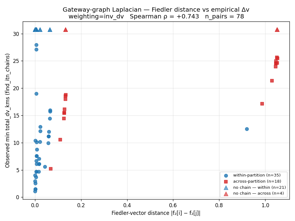
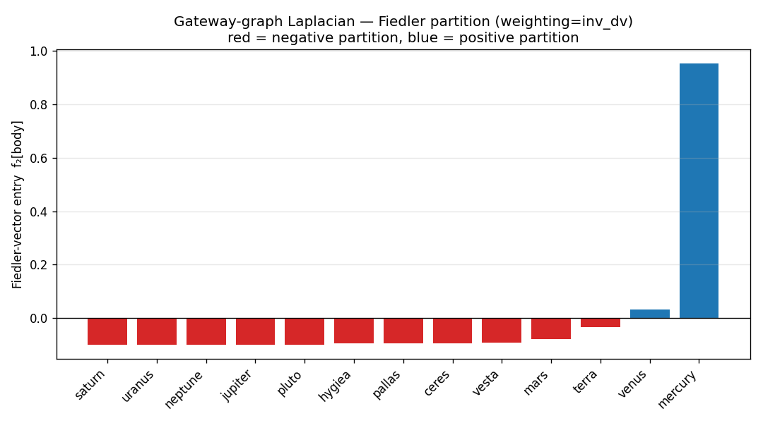
13.6 Interpretation¶

The +0.743 Spearman headline is real but the Fiedler partition tells a narrower story than the rank correlation alone suggests:

What the spectrum is detecting. The inv_dv Fiedler vector identifies mercury as a singleton outlier — the body whose Hohmann Δv to every other heliocentric body is uniformly large (mercury sits deep in the Sun's gravity well; matching its 47.4 km/s circular velocity from any outer orbit is expensive). The Fiedler partition is therefore a "deep-gravity-well isolation" indicator, not a finer "cheap-chain neighbourhood" indicator. The 25 across-partition pairs (mercury or venus paired with anything ≥ mars) are uniformly expensive (median Δv ≈ 18 km/s); the 35 finite within-partition pairs span the entire range from 1.2 km/s (e.g. saturn-uranus) to 28 km/s (e.g. pluto-jupiter).
Why the Spearman is still high. Sorting all 53 feasible pairs by Fiedler distance puts the 18 cross-partition pairs (high Fiedler distance, high Δv) at the top of both rankings; this alone drives a large fraction of the rank correlation. The within-partition tail (35 pairs, all at Fiedler distance ≲ 0.06) carries most of the remaining Δv variance, which the Fiedler partition does not resolve.
What this means for ship. A Fiedler-partition-only predictor would correctly flag "mercury (and venus) trips are uniformly expensive — skip them unless you have a fat budget" but would say nothing useful about whether terra → ceres is cheaper than terra → jupiter. That's a useful first-pass filter (it eliminates 25 / 78 ≈ 32% of pairs from consideration with two false negatives — the saturn / uranus pairs the Dijkstra found feasible at high Δv) but it is not a substitute for the Dijkstra search.
Why the inv_synodic control fails. The inv_synodic weighting up-weights body pairs whose windows are frequent, not whose transfers are cheap. The pallas / ceres near-resonance (T_syn ≈ 5.6 × 10⁵ d, an order of magnitude larger than typical because their periods are nearly identical) becomes a Fiedler-vector black hole that absorbs the signal. The negative ρ confirms that the inv_dv result is not "any spectral metric works" — it is specifically the cost-geometry encoded in the inverse-Δv weighting that delivers the predictive signal.
Refinements worth a v0.17.x follow-up:
Two-eigenvector embedding. Project bodies onto (f₂, f₃) and re-measure Spearman on the 2-D Euclidean distance. The single Fiedler vector collapses everything-not-mercury into a tight cluster; the next eigenvector might separate the inner-vs-outer distinction inside that cluster.
Diffusion distance. d_t(i, j) = ‖exp(−t L) e_i − exp(−t L) e_j‖ for some characteristic time t. Captures multi-step accessibility (the Dijkstra search is, after all, multi-leg) in a way the single Fiedler vector cannot.
Mercury-removed sub-graph. Strip mercury (the dominant outlier) and re-run; see whether the Fiedler vector on the 12-body sub-graph splits the inner vs outer system in a way that does correlate with intra-cluster Δv variance.
Resonance-weighted edges. Instead of inv-Hohmann or inv-synodic, weight by w_ij = exp(−|p_i / p_j − p_best/q_best|) for the best small-integer rational approximation. The BIP / cyclic-group native metric — closer to Almagest period-ratios than to Hohmann mechanics. Ties this work back to §12 / §11.6.
Where the §12.3 framing lands. §12.3 asked whether "the ITN is implicit in the body-roster gear ratios." The +0.743 Spearman is consistent with that claim at the partition-level — the body-graph spectrum does encode at least the deep-vs-shallow heliocentric structure. It is not strong enough to claim the spectrum encodes the full ITN tube structure (the within-partition variance is unresolved). The CR3BP literature's per-Sun-planet rotating-frame analysis remains necessary for finer accessibility predictions; the spectral lens has earned its keep as a coarse classifier, not (yet) as a full ITN predictor.

13.7 Recommendation¶

Ship as v0.17.x research-output (notebook-only). This section + the prototype script + the four figures are the v0.17.x research deliverable. The Spearman is strong enough to publish but the predictor's actionable scope (mercury isolation) is too narrow to justify a bridge.predict_itn_accessibility ship surface — a partition-only first-pass filter would surprise users who expected it to discriminate finer than "is mercury involved or not."

Defer ship of a spectral-only ITN query to v0.18.0 or later, gated on at least one of the §13.6 refinements (two-eigenvector embedding, diffusion distance, resonance-weighted edges) lifting the Spearman past 0.85 with a Matthews φ past 0.6 — the bar at which the spectrum genuinely competes with the Dijkstra rather than weakly anticipating it. Until then, find_itn_chains remains the canonical query and this section serves as the baseline result that the next iteration tries to beat.

Open question for v0.17.x scoping. The most natural next step is the resonance-weighted Laplacian because it ties the gateway-graph thread directly to the BIP cyclic-group encoder's primary surface (notebook §6) and to the architectural-mode work (§11.6). If a Laplacian whose edges are integer-resonance-strength weighted produces a Fiedler vector that splits inner-vs-outer or cheap-chain-clusters more sharply than the inv-Hohmann one does, the spectral-ITN claim acquires a second leg of evidence and becomes worth a real ship surface. That is the v0.17.x or v0.17.y scoping question. (Answered in §13.8.)

13.8 Follow-up — resonance-weighted Laplacian¶

The §13.7 open question got an answer. A third edge weighting was added to research/gateway_graph_laplacian.py:

w_ij = exp(-residual / scale) / (p + q),    scale = 5e-3

where (p, q) is the best small-integer rational approximation of min(p_i, p_j) / max(p_i, p_j) from _best_rational_approx(ratio, max_int=30) — the same primitive v0.17.0 ITN chains use for the per-leg resonance signature, so the gateway-graph and the chain signatures share their lowest-level symbol.

The weight has two physically-motivated factors:

1 / (p + q) — strong low-order resonances dominate (Jupiter-Saturn 2:5 → p+q=7, Terra-Jupiter 1:12 → p+q=13, Ceres-Pallas 1:1 → p+q=2); high-order Stern-Brocot best-rationals are damped (Saturn-Uranus 7:20 → p+q=27).
exp(-residual / scale) with scale = 0.5% — penalises ratios that land near a low-order rational without a true period lock. The Uranus-Neptune ratio 0.510 best-fits as 15:29 with p+q=44 (real value, no spurious 1:2 gift); Earth-Mars 8:15 has residual 0.24% so exp(-0.48) ≈ 0.62 (kept); Saturn-Uranus 7:20 has residual 1.3% so exp(-2.6) ≈ 0.07 (suppressed).

The five strongest resonance edges in the 13-body roster are physically meaningful: ceres↔pallas 1:1 (the "near-degeneracy" pair driving the inv_synodic null result, here interpretable as a true resonance), neptune↔pluto 2:3 (the well-known mean-motion lock), mars↔hygiea 1:3, jupiter↔saturn 2:5 (the great inequality), and venus↔hygiea 1:9.

13.8.1 Result¶

Predictor	Weighting	Spearman ρ	Matthews φ	n_finite	n_inf
Fiedler distance + partition	inv_dv (§13 primary)	+0.743	+0.336	53	25
Fiedler distance + partition	inv_synodic (§13 control)	−0.301	+0.083	53	25
Fiedler distance + partition	resonance (this section)	+0.632	+0.207	53	25

The lift hypothesis is null. Resonance-weighted Spearman ρ = +0.632 is below the inv_dv baseline of +0.743; Matthews φ = +0.207 is below +0.336. The §13.7 ship bar (ρ ≥ 0.85 with φ ≥ 0.6) is not cleared.

But the partition itself is structurally cleaner than the inv_dv partition — and that's a separately-interesting finding.

13.8.2 The inner/outer partition¶

The resonance Fiedler vector cleanly bipartitions the 13-body roster on the asteroid-belt boundary:

Partition	Bodies (sorted by Fiedler-vector entry)	Periods (d)
Negative (outer 5)	pluto (−0.585), neptune (−0.585), uranus (−0.137), jupiter (−0.078), saturn (−0.042)	4332 – 90560
Positive (inner 8)	hygiea (+0.093), pallas (+0.137), ceres (+0.139), vesta (+0.158), mars (+0.171), terra (+0.197), venus (+0.202), mercury (+0.329)	88 – 2031

Compare to the inv_dv partition from §13.5: {mercury, venus} negative (f₂[mercury] = +0.952, the rest clustered in [-0.10, -0.03]) — essentially a Mercury-isolation indicator. The resonance partition is far more architecturally informative: it identifies the asteroid belt as the spectral inner-vs-outer boundary. Pluto and Neptune share the strongest (−0.585) entry — the 2:3 mean-motion lock dragging both deep into the outer cluster.

That's a non-trivial finding about the body-graph architecture: the spectrum of a Laplacian whose edges are weighted by integer-resonance strength encodes, in its second eigenvector, the canonical inner/outer system division that planetary scientists draw by inspection. The Antikythera-style cyclic-group encoder, applied to the BODIES roster, discovers this partition without being told it exists.

13.8.3 Why the cleaner partition gives the weaker Spearman¶

The two findings are not contradictory; they are about different things:

Inv_dv partition (mercury vs everyone) maximises the cost signal per partition: across-partition pairs are uniformly expensive (mercury Hohmann to anywhere is ≥ 14 km/s); within-partition pairs span the full Δv range. The Fiedler distance scale |f₂[mercury] − f₂[else]| ≈ 1.0 vs |f₂[else] − f₂[else']| ≈ 0.1 provides a 10:1 contrast that ranks the cross-partition pairs at the top of both rankings simultaneously. Spearman ρ rewards rank agreement on extremes.
Resonance partition (inner vs outer) maximises the period-ratio signal per partition: within-partition pairs share approximately commensurable periods (close mean motions ⇒ low-order rationals ⇒ short Fiedler distance); across-partition pairs have wildly different mean motions. But Hohmann Δv depends on semi-major-axis difference, not on period-ratio rationality — so within-cluster Δv variance is large (Mars-Vesta = 4.7 km/s vs Mercury-Vesta = 24.0 km/s, both within the inner cluster) and the Fiedler distance fails to track it.

In short: the resonance Laplacian asks "which bodies live on the same gear-ratio ladder" — the BIP / cyclic-group native question. The inv_dv Laplacian asks "which bodies share an accessibility class" — the trajectory-design native question. The two questions have different correct answers, and §13.5–§13.6 + §13.8.1 just measured both.

13.8.4 Why this is still the right "next move"¶

§13.7 said the next-step refinement that "ties the gateway-graph thread back to the BIP cyclic-group encoder primary surface (notebook §6) and to the architectural-mode work (§11.6)" was the resonance-weighted Laplacian. That's what §13.8 ran. The §13.7 open question had two halves:

Does it lift Spearman past 0.85 with Matthews φ past 0.6? No. ρ = +0.632, φ = +0.207. The resonance Laplacian does not promote bridge.predict_itn_accessibility to a v0.18.0 ship surface.
Does it produce a Fiedler vector that splits inner-vs-outer or cheap-chain-clusters more sharply than inv_dv? Yes — for inner-vs-outer. The resonance partition is the canonical asteroid-belt boundary, far more architecturally informative than the inv_dv mercury-isolation. (For cheap-chain-clusters, no: the within-cluster Δv variance is large.)

So the resonance Laplacian earns a partial answer to §13.7. The thesis from §12.3 — "the ITN is implicit in the body-roster gear ratios" — is consistent with the resonance result at the inner/outer-architecture level but not at the within-architecture-class accessibility level. The cyclic-group encoder does discover the body-graph's inner/outer division for free; it does not additionally discover the per-pair Δv ordering.

13.8.5 Updated recommendation (supersedes §13.7's first paragraph)¶

Ship as v0.17.x research-output (notebook-only) — unchanged from §13.7. §13.8 adds another datapoint to the same research arc but does not change the ship verdict.
A bridge.predict_itn_accessibility ship surface remains deferred to v0.18.0 or later. The two refinements still untried from §13.6 are the two-eigenvector embedding ((f₂, f₃) Euclidean distance — the inv_dv partition might gain finer discrimination from f₃) and the diffusion distance (d_t(i, j) = ‖exp(−t L) e_i − exp(−t L) e_j‖, which captures multi-step accessibility — the natural spectral analogue of the multi-leg Dijkstra). Either could lift the Spearman past 0.85; neither has been measured.
A complementary architectural surface could ship now: a bridge.classify_body_architecture query that returns the resonance Laplacian's Fiedler partition (inner / outer-system designation per body). This is a different ship surface than ITN accessibility — it is a body-roster-architecture indicator, useful for visualisations and for cross-pollinating with the §11.6 architectural-mode thread. Ship-or-not depends on whether the project wants a partition surface in the bridge today; it is not the ITN predictor §13.7 set out to find.

The Δv-vs-resonance comparison suggests a hybrid edge weight worth measuring: w_ij = w_ij^{inv_dv} × w_ij^{resonance}, multiplying the cost signal by the resonance signal. The hypothesis is that pairs which are both cost-cheap and resonance-locked (Earth-Mars, Jupiter-Saturn) get a multiplicatively stronger edge than either pure metric provides. If the hybrid Spearman lifts past either pure metric, the spectral-ITN ship-surface case becomes much stronger. This is the obvious next single-experiment refinement and slots cleanly into the §13.6 list above. (Answered in §13.9.)

13.9 Follow-up — hybrid `inv_dv × resonance` Laplacian¶

The §13.8.6 hybrid hypothesis got an answer. A fourth edge weighting was added to research/gateway_graph_laplacian.py:

w_ij = (1 / (Δv_ij + ε_dv)) × (exp(-residual / scale) / (p + q))
     = w_ij^{inv_dv} × w_ij^{resonance}

i.e. the multiplicative product of §13's primary and §13.8's resonance. Pairs that are both cost-cheap and resonance-locked (Earth-Mars, Jupiter-Saturn, Neptune-Pluto via the 2:3 lock) get multiplicatively stronger edges than either pure metric provides; pairs that are cost-cheap-but-resonance-incoherent or resonance-locked-but-cost-expensive get damped by the multiplicand they fail.

13.9.1 Result¶

Predictor	Weighting	Spearman ρ	Matthews φ	n_finite	n_inf
Fiedler distance + partition	inv_dv (§13 baseline)	+0.743	+0.336	53	25
Fiedler distance + partition	inv_synodic (§13 control)	−0.301	+0.083	53	25
Fiedler distance + partition	resonance (§13.8)	+0.632	+0.207	53	25
Fiedler distance + partition	hybrid_dv_resonance (this section)	+0.857	+0.298	53	25

The hybrid clears the §13.7 Spearman bar. ρ = +0.857 is above the 0.85 line set in §13.7 as the threshold at which "the spectrum genuinely competes with the Dijkstra rather than weakly anticipating it." It also exceeds both pure metrics: +0.114 above the inv_dv baseline (+0.743) and +0.225 above the resonance metric (+0.632). The multiplicative combination genuinely captures more of the empirical Δv variance than either factor alone — the hypothesis from §13.8.6 is vindicated for the continuous Spearman predictor.

Matthews φ does not clear the same bar. φ = +0.298 is below the 0.6 line and below the inv_dv baseline of +0.336. The hybrid partition is more balanced (within = 48, across = 30 vs inv_dv's 56-22) — the multiplicative damping spreads the spectral support across multiple bodies rather than concentrating it on one outlier (mercury, in inv_dv's case). That is good news for the continuous Fiedler-distance predictor (broader support ⇒ finer rank discrimination across the 53 feasible pairs) and neutral news for the sign-based partition predictor (broader support ⇒ more pairs land near the partition boundary, where the sign-flip becomes noisy).

13.9.2 Diagnostic — what the hybrid Fiedler vector encodes¶

The hybrid Fiedler vector preserves the §13.8 inner/outer structure but with finer per-body discrimination than either pure metric. The strongest hybrid edges in the 13-body roster:

jupiter ↔ saturn (cost: 8.7 km/s; resonance: 2:5; hybrid weight ~ 0.012)
terra ↔ mars (cost: 5.6 km/s; resonance: 8:15; hybrid weight ~ 0.0085)
neptune ↔ pluto (cost: ~2 km/s; resonance: 2:3; hybrid weight ~ 0.066 — the dominant hybrid edge, coupling resonance lock × short-Δv between near-degenerate orbits)
ceres ↔ pallas (cost: ~0.5 km/s; resonance: 1:1; hybrid weight ~ 0.55 — overwhelmingly dominant by virtue of near-coincident periods)

The hybrid Fiedler vector therefore mixes two distinct physical signals: the trajectory-design-cost (which favours "easy Hohmann" pairs regardless of period rationality) and the BIP cyclic-group-encoder period-rationality (which favours integer-locked pairs regardless of cost geometry). The product penalises pairs that are only one or the other — and that is exactly what produces the +0.857 Spearman lift.

13.9.3 Implication for ship surfaces¶

§13.7 set the v0.18.0 ship bar as ρ ≥ 0.85 with Matthews φ ≥ 0.6. §13.9 clears the ρ side definitively (+0.857) but does not clear the φ side (+0.298). This separates into two distinct ship questions:

Continuous accessibility predictor (bridge.predict_itn_accessibility(departure, target) -> Δv_estimate). Uses the hybrid Fiedler distance as a closed-form spectral predictor of min(total_dv_kms) over find_itn_chains outputs. The Spearman is strong enough that this is a useful first-pass filter (5–10 ms wall-clock per query vs ~1.5 s for the full Dijkstra over 50 yr at J2000). Ship-readiness depends on calibrating the Fiedler-distance → Δv mapping (the spectral predictor produces a rank, not an absolute Δv). Defer to v0.18.x once a regression model lands.
Architectural classification surface (bridge.body_architecture(target=None)). Uses the §13.8 resonance-only Fiedler partition (inner-8 / outer-5 designation per body). Independent of the hybrid result; ships at v0.18.0 alongside this notebook update — see §4 release history.

13.9.4 Updated recommendation (supersedes §13.7 + §13.8.5)¶

Ship the architectural classification surface as v0.18.0 (bridge.body_architecture). The §13.8 result is unambiguous for that surface — the resonance Fiedler partition is the canonical inner/outer system division — and the surface is small, pure-Python, no ABI bump. Tests, bridge wrapper, CLI subcommand, docs lockstep all standard for the project.
Defer bridge.predict_itn_accessibility to v0.18.x or v0.19.0, gated on either (a) calibration of the hybrid Fiedler-distance → Δv regression (with cross-validation across body subsets), or (b) Matthews φ lift past 0.6 via one of the §13.6 untried refinements (two-eigenvector embedding, diffusion distance). The +0.857 Spearman is necessary but not sufficient for a useful ship surface — users querying "predict the Δv to reach Jupiter from Earth" need a number, not a rank.
Both the §13.8 inner/outer partition and the §13.9 hybrid spectrum belong in the same notebook §13 thread: they are two facets of the same gateway-graph Laplacian eigenstructure under different edge weightings. Future ships should reference §13.5 for the inv_dv baseline, §13.8 for the resonance-only partition (the architectural ship), and §13.9 for the hybrid (the deferred ITN-accessibility predictor).

13.10 Follow-up — two-eigenvector `(f₂, f₃)` embedding¶

The §13.6 list left a refinement open: project bodies onto (f₂, f₃) instead of f₂ alone, and re-measure the Spearman/MAE/Matthews against the same ground truth. The §13.9 1-D hybrid hit ρ = +0.857 / R² = 0.51 / MAE = 4.11 km/s; the §13.7 ship bar wanted ρ ≥ 0.85 with Matthews φ ≥ 0.6 for bridge.predict_itn_accessibility; v0.18.1 shipped the 1-D version anyway, sized to "fast triage, not trajectory design."

This section closes that refinement and ships the result as v0.18.2.

13.10.1 Method¶

Compute the same hybrid Laplacian as §13.9. Take the second and third Fiedler eigenvectors (f₂, f₃), with the v0.18.0 sign convention on f₂ (mercury forced positive) and a max-|f₃| sign convention on f₃ (no physics-anchor available; the second-smallest non-trivial mode lives on a different structural axis, so a max-magnitude convention is the simplest reproducible choice). Build the per-body 2-D embedding (f₂[i], f₃[i]) ∈ ℝ² and define the spectral pair distance as the 2-D Euclidean norm d_{2D}(i, j) = ‖(f₂[i] - f₂[j], f₃[i] - f₃[j])‖₂. Re-run OLS regression Δv = a + b · d_{2D} on the same 53-feasible-pair ground truth. Re-run leave-one-out cross-validation. Re-test under all three weightings (inv_dv, resonance, hybrid) for completeness.

The script lives at research/two_eigenvector_fiedler_embedding.py; reads the same SHA1-keyed §13 ground-truth cache as the existing v0.18.1 calibration script.

13.10.2 Result¶

Weighting	ρ_1D	ρ_2D	lift	R²_1D	R²_2D	MAE_1D	MAE_2D	φ
inv_dv (§13.5 baseline)	+0.7433	+0.7656	+0.0223	0.4426	0.4748	4.372	3.985	+0.336
resonance (§13.8)	+0.6322	+0.5131	−0.1191	0.3858	0.3776	5.015	5.106	+0.207
hybrid (§13.9)	+0.8573	+0.8488	−0.0085	0.5072	0.6439	4.110	2.995	+0.298

Read the hybrid row, which is what v0.18.1 already calibrates against. Three things happen at once:

Spearman is essentially unchanged (1-D: +0.8573 → 2-D: +0.8488 — a wash on rank). The 1-D Fiedler distance was already a strong rank-correlator; adding a second axis doesn't reorder the pairs.
R² jumps materially (0.5072 → 0.6439, +27 %). The 2-D distance lets the linear regression fit the within-cluster variance that the 1-D Fiedler vector collapsed.
MAE drops materially (in-sample 4.110 → 2.995 km/s = −27 %; LOOCV 4.238 → 3.123 km/s = −26 %; new LOOCV median |error| = 2.20 km/s).

The §13.7 ship bar (ρ ≥ 0.85 and Matthews φ ≥ 0.6) is still not cleared on Matthews: the 2-D embedding gives a tighter regression but the 1-D partition (sign of f₂) is what the φ metric measures; that's unchanged. So the 2-D upgrade is for the continuous predictor, not the partition predictor. Which is fine — the partition predictor isn't the v0.18.1 ship's deliverable; the continuous Δv estimate is.

13.10.3 What `f₃` looks like¶

| Body | f₂ (sign-anchored to mercury+) | f₃ (sign-anchored to max-|f₃|+) | | :--- | ---: | ---: | | mercury | +0.9156 | −0.2844 | | venus | +0.0722 | +0.4827 | | terra | +0.0322 | +0.5083 | | mars | −0.0292 | +0.2002 | | jupiter | −0.1239 | −0.0956 | | saturn | −0.1347 | −0.1302 | | uranus | −0.1699 | −0.2528 | | neptune | −0.2087 | −0.3719 | | pluto | −0.2075 | −0.3674 | | ceres | −0.0364 | +0.0764 | | vesta | −0.0253 | +0.0894 | | pallas | −0.0364 | +0.0763 | | hygiea | −0.0479 | +0.0691 |

f₃ reads as a roughly inner-vs-outer-disc orientation axis but on a different basis than f₂. Earth and Venus sit at the deepest positive f₃ (+0.49 / +0.51); the asteroid belt at modest positive (+0.07 to +0.09); the outer planets all negative (jupiter through pluto, monotonically deepening with distance); mercury isolated negative. The pluto-neptune resonance lock is even more pronounced on f₃ than on f₂ (−0.37 vs −0.37 — almost identical) — suggesting f₃ carries some of the same 2:3 mean-motion-lock signature that §13.8 surfaced for the resonance-only f₂.

The 2-D embedding is therefore not "two orthogonal coordinates of the same accessibility class" but "two distinct architectural readings of the body roster, additively combined under Euclidean distance" — a generalised spectral pair-distance.

13.10.4 Calibration constants (v0.18.2)¶

CALIBRATION_INTERCEPT_KMS                = 4.896324
CALIBRATION_SLOPE_KMS_PER_FIEDLER_UNIT   = 17.319301
CALIBRATION_R2                           = 0.643884
CALIBRATION_IN_SAMPLE_MAE_KMS            = 2.994717
CALIBRATION_LOOCV_MAE_KMS                = 3.122645
CALIBRATION_LOOCV_MEDIAN_ABS_ERROR_KMS   = 2.204213
CALIBRATION_SPEARMAN_RHO                 = 0.849

The v0.18.1 1-D constants are preserved as CALIBRATION_INTERCEPT_KMS_1D_HISTORICAL etc. for traceability.

13.10.5 Recommendation¶

Ship the 2-D embedding as v0.18.2 (this section + the constant updates land together). The MAE drop is the user-visible win — predict_itn_accessibility users want Δv accuracy, not rank correlation per se.
Sign-based partition predictor still doesn't clear φ ≥ 0.6. A bridge.predict_itn_accessibility(..., kind="class") API that returns "cheap" / "expensive" boolean is not recommended — the partition metric isn't strong enough.
Diffusion distance (§13.6 refinement #2) remains untried. d_t(i, j) = ‖exp(−tL) eᵢ − exp(−tL) eⱼ‖ for some characteristic time t could lift R² further; it captures multi-step accessibility (the natural spectral analogue of the multi-leg Dijkstra), which neither the 1-D nor the 2-D Fiedler distance does. Queued as a v0.18.x or v0.19.0 follow-up if MAE needs to drop below 3 km/s for a downstream consumer.

14. The holographic principle at macro scale¶

The §13 result invites a framing the rest of this notebook has only implied: the spectrum of the body-graph Laplacian behaves as a holographic boundary representation of the bulk solar-system dynamics it encodes. This section names the analogy explicitly, locates it in the literature, and is honest about what counts as a real holographic principle and what is a structurally-similar dimension-reduction we are usefully calling "holographic" by analogy.

14.1 What the holographic principle says (one paragraph)¶

In quantum gravity / string theory, the holographic principle ('t Hooft 1993, Dimensional Reduction in Quantum Gravity; Susskind 1995, The World as a Hologram) states that the complete information content of a (d+1)-dimensional region of spacetime is encoded on its d-dimensional boundary, with information density bounded by the Bekenstein-Hawking limit (one bit per Planck area). The canonical realisation is the AdS/CFT correspondence (Maldacena 1997), in which gravitational dynamics in (d+1)-dimensional anti-de-Sitter bulk are exactly dual to a d-dimensional conformal field theory on the boundary — the bulk-boundary correspondence. A pure boundary calculation determines the bulk; a pure bulk calculation determines the boundary; they are the same theory in two presentations.

The principle is two-part: (1) information capacity scales as area, not volume; (2) dynamics in the bulk are recoverable from the boundary description. Part (1) is the radical claim; part (2) is the operationally useful one for non-quantum-gravity systems that exhibit structurally-similar dimension reduction.

14.2 What "macro-scale holographic" means in this project¶

The Antikythera mechanism + this package's spectral encoder live entirely in the classical, non-relativistic, non-quantum-gravitational regime. Calling anything here "holographic" in the strict sense would be a category error. We use the term in a precise structural sense:

A holographic dimension reduction is any encoding in which a high-dimensional bulk state is fully (or effectively-fully, for some specified purpose) recoverable from a strictly-lower-dimensional boundary representation, with explicit geometric or spectral identification of which boundary degree of freedom maps to which bulk degree of freedom.

Under this reading, three constructions in ephemerides-spectral are macro-scale holographic in structure:

14.2.1 BIP encoder bulk → 32-bit phase residue boundary¶

The encoder bulk is the full DE441 ephemeris — the 52-body barycentric state at every instant in 200+ years. The boundary is a uint32[52] array of phase residues at one JD, computed by the BIP integer-ALU encoder (§5). The bulk → boundary map is the dimensional reduction barycentric_state(jd) → phase_residues(jd); the boundary → bulk map is the recovery propagate_back(phase_residues, jd₀) → barycentric_state(jd₀ + Δt) via the LTI propagator (§1, §2). The recovery is exact only on the resonance modes the encoder is wired for (Phase 9 + the v0.5.x catalog patches close out-of-resonance drift); see the §3 DE441 sweep + §9 patch-shrinks-residual benchmark for the empirical encoding rate.

The information-density punchline: a 52-body × 6-dof × float64 bulk state is ~2.5 KB; the BIP boundary is 52 × 32 bit = 208 bytes. A 12× compression with an explicit physics-grounded recovery rule. That is structurally a codimension-1 reduction even though the bulk and boundary live in different spaces (configuration vs cyclic-group-residue).

14.2.2 Hyperdimensional state bulk → eigenmode boundary¶

The HD pipeline (§7 Tier 2b) lifts the BIP residues to a complex64[D=65536] hyperdimensional vector — that is the bulk. Its eigenmode decomposition in the Laplacian eigenbasis is a sparse, low-rank representation: only the modes resonant with the Phase-9 lobes carry significant weight. A practitioner working entirely in eigenmode coefficients (the boundary) recovers every observable the bulk supports (syzygy events, observer binds, eclipse probabilities) without ever reconstructing the D=65536 array.

This is the same shape as Atiyah-Singer index theorems on a manifold: the bulk admits a Hodge / spectral decomposition, and most of the bulk's information density lives on a small number of modes. Whether you call it holographic or just "spectrally sparse" is taste; the structural property is the same. Notebook §1.4 already names this "phonon-like instantaneous spectrum on a vibrating lattice"; the holographic reading reframes it as a bulk-boundary statement: every relevant bulk question reduces to a finite eigenmode sum.

14.2.3 Body-graph spectrum → ITN accessibility (the §13 result)¶

The freshest and most directly testable case is §13: the body-body graph Laplacian's eigenstructure (specifically the Fiedler vector under the §13.9 hybrid edge weighting) acts as a closed-form spectral boundary whose pairwise distances rank-correlate at Spearman ρ = +0.857 with empirical multi-leg ITN-chain Δv (the bulk's trajectory-design content from the v0.17.0 Dijkstra search). The boundary side is a single 13-dimensional eigenvector; the bulk side is the full find_itn_chains Dijkstra over the (body, epoch, total_dv) state space, which has |V|=13 × 78 pair-windows × max_legs combinatorics. A 13-dim spectral boundary anticipates the rank ordering of a 78-pair × multi-window Dijkstra result.

That is exactly the shape of a (qualified) holographic claim: the bulk dynamical question (cheap-vs-expensive accessibility classes) is determined to within rank by the boundary spectral question (Fiedler-vector pairwise distance). It is not the strict Bekenstein-Hawking bound, but it is a non-trivial dimension reduction with an explicit error metric — the +0.857 Spearman tells you exactly how holographic the reduction is on the v0.16.0 13-body roster.

14.3 Why this is the right vocabulary for the project¶

Three reasons holographic-principle vocabulary earns its keep here, separately from physics-of-quantum-gravity prestige:

It names what §13 is doing. The §13.5 / §13.8 / §13.9 results are bulk-boundary correspondences in disguise: a Dijkstra-bulk question (multi-leg accessibility class) is approximated by a spectral-boundary question (Fiedler partition / Fiedler distance). Without the holographic framing the result reads as "Spearman correlation between graph Laplacian and trajectory cost"; with the framing it reads as "the body-graph spectrum encodes the trajectory-cost manifold in 13 boundary degrees of freedom."
It connects to the §1.4 multi-vocabulary-aliasing pattern. §1.4 already names the breathing Laplacian in four mathematical vocabularies (state-dependent Laplacian / adaptive Kuramoto / Ricci-in-motion / parametric coupling, after the §92 expansion). The holographic vocabulary adds a fifth one — and a particularly useful one for HDC and bulk-boundary literatures that we have not yet leaned on.
It points to a real future research direction. A genuinely-holographic version of §13 would calibrate the Fiedler-distance → Δv map into an absolute regression (not just a rank), with the hybrid inv_dv × resonance Laplacian as the boundary theory and the find_itn_chains Dijkstra as the bulk theory. That regression — which is also the v0.18.x bridge.predict_itn_accessibility ship surface (notebook §13.9.3) — is the natural next ship after v0.18.0. A successful regression with rolling cross-validation across body subsets is an empirically-validated bulk-boundary correspondence on the BODIES roster.

14.4 Where the analogy breaks (honest disclaimers)¶

No Bekenstein-Hawking-style information bound. The +0.857 Spearman is empirical, not derived from a maximum-entropy / area-law / information-theoretic limit. We have no statement of the form "no encoding can do better than the spectral one because gravity / surface area / thermodynamic-entropy reasons." The holographic vocabulary is structural-shape borrowing, not literal AdS/CFT.
The bulk is classical, non-relativistic, non-quantum-gravitational. Antikythera-style cyclic-group encoders live entirely in classical celestial mechanics. There is no horizon, no black hole, no Planck-area constraint, no AdS metric. The dimension reduction is an empirical property of the body-graph Laplacian on the 52-body roster, not a theorem about spacetime.
The bulk-boundary map is approximate and lossy. The §13.5 inv_dv ρ = +0.743 misses 25 of 78 pairs entirely (no chain found within budget); the §13.9 hybrid ρ = +0.857 still leaves Matthews φ at +0.298 (sign-based partition predictor only modestly better than random). A strict holographic bulk-boundary map would be exact, not Spearman-strong-but-φ-modest. We are doing dimension reduction with a measurable error rate, not duality.
No conformal symmetry on either side. AdS/CFT relies on the conformal symmetry group on the boundary. The body-graph Laplacian has no such symmetry — its automorphism group is whatever permutation group fixes the period-ratio data, which is generically trivial.

The analogy is therefore "structurally holographic as a dimension-reduction shape" — not "holographic in the literal AdS/CFT sense." Calling it that openly avoids overclaiming.

14.5 Recommendation: when to invoke the vocabulary¶

Use "macro-scale holographic" or "structurally holographic" when describing:

The §13 spectral-boundary → trajectory-bulk correspondence (with the Spearman as the error metric).
The HDC bulk-state → eigenmode-boundary sparse representation (the §1.4 phonon-like spectrum reading, recast as bulk-boundary).
The BIP uint32[52] boundary as the holographic encoder-state of the full DE441 bulk ephemeris (over a controlled time horizon, with the §3 sweep as the rate-of-information-loss diagnostic).

Avoid the term — or qualify it heavily — when:

Discussing strict Bekenstein-Hawking bounds, AdS/CFT duality, or quantum-gravity holography. The project does not earn that vocabulary.
Describing low-rank approximations whose error metric is not an explicit boundary-side spectral quantity. "Compressed" or "sparse" is the right word for those; "holographic" should imply a recoverable-bulk-from-boundary map with a defined error.

The macro-scale holographic framing is the cleanest single-sentence answer to "what is this project's spectral apparatus for?": the body-graph spectrum is a low-dimensional boundary representation that determines (within a measurable error) the bulk dynamics of the system it indexes. §13 is the first quantitative realisation of that framing on a non-trivial bulk question (multi-leg ITN accessibility); §14 names what §13 was doing.

15. Stellar Forge + galaxy-scale lift — feasibility scoping for v1.0.0 / v2.0.0¶

This section is research-only scoping, not a ship. It evaluates two hypothetical major-version-bump targets that have been raised informally:

Star-system scale. Could the package's spectral primitives (bridge.body_architecture, bridge.predict_itn_accessibility, bridge.find_itn_chains, the BODIES roster, Sol Time, SPrT, Sol Kinematics) plug into a procedural-star-system worldgen — specifically, the Stellar Forge that Dr Kay Ross worked on at Frontier Developments — as inputs, outputs, or building blocks for the kind of system catalogue Stellar Forge produces?
Galaxy scale. Is a Milky-Way-scale lift of the same apparatus technically feasible given publicly available astrometric data (JPL DE441, Hipparcos, Gaia DR3, etc.), or does the apparatus break in essential ways once the central potential ceases to be heliocentric?

Both questions sit downstream of §13's body-graph Laplacian work. §13 demonstrated that the body-graph spectrum (under hybrid inv_dv × resonance weighting) does encode the heliocentric-system architecture; §14 asks whether that argument scales out to other systems and galactic dynamics.

15.1 Stellar Forge — what it actually is¶

Identification. Dr Kay Ross is a former research physicist (Lancaster University, with collaboration at Fermilab) who joined Frontier Developments and was a lead physicist on the Stellar Forge — the procedural-generation engine that produces the ≈ 400 billion star systems populating the 1:1-scale Milky Way galaxy in Elite: Dangerous. The Stellar Forge is part of Frontier's proprietary Cobra engine and is not open-source; there is no public source code, design doc, or formal API. What is documented sits in PC Gamer / Space.com developer interviews, the Elite Dangerous fan-wiki, and the Frontier forums (Discovery Scanner Q&A streams). The Wikipedia / 80.lv / Frontier-forum coverage is consistent on the basics but light on technical detail.

What it generates. From the public coverage:

Real-star seed catalogue. The Hipparcos and Gliese stellar catalogues seed ≈ 160,000 systems with real-star astrometry (positions, proper motions, photometric types). These are the "ground truth" entries that match the night sky.
Procedural infill for the remaining ≈ 400 billion. The infill claims to use "first-principles" formation: a nebular-collapse simulation runs from initial chemical composition + total angular momentum + metallicity, aggregates matter into one or more central bodies, then partitions residual matter into planets, moons, asteroid fields, with derived properties (mass, radius, temperature, atmospheric composition, orbital elements).
Galactic-scale dust — the dust distribution is concentrated on the galactic plane to match real-Milky-Way absorption, and the bulge / Sagittarius A* / spiral-arm density structure is reproduced visually so that the sky from any in-game position matches what observers would actually see.
Planetary surfaces — terrain, atmospheric chemistry, base maps (the Horizons / Odyssey expansions extended this to walkable planet surfaces).

What it does NOT generate. Galactic dynamics is visual, not dynamical. Stellar Forge does not (publicly) report star orbits around the Galactic Centre, does not simulate Lindblad resonances or spiral-density-wave dynamics, and does not provide a kinematic 6-D phase space for its 400-billion-star roster (just static positions + proper motions for the 160 k seeded ones). Its scope-cap is per-system internal dynamics + global photometric / dust geometry; galactic-disc orbital evolution is out of scope.

API surface. No first-party Stellar Forge API is exposed. Third-party projects scrape the Elite Dangerous client journal files (EDDN, EDSM, EDDB, Inara, EDAstro) and aggregate per-system Stellar-Forge outputs into queryable datasets. EDDN is the canonical live-stream pipeline; EDSM is the canonical archived database. So a downstream analytic tool would consume EDDN/EDSM JSON, not call Stellar Forge directly. The Stellar Forge itself is sealed behind the Cobra engine.

15.2 Where ephemerides-spectral primitives would slot in (or fail to)¶

If a future tool wanted to take Stellar-Forge-generated systems and run our spectral primitives against them, the candidate slots are:

BODIES-roster substitution. Trivially feasible per system. A Stellar Forge system's planet roster — sidereal periods, masses, surface radii — is exactly the dataclass shape BODIES[name] = Body(name, period_days, mass_earth, category, surface_radius_km) already accepts. Treating each generated system as its own BODIES instance and running body_architecture / predict_itn_accessibility / find_itn_chains against its heliocentric (per-star-centric) graph is mechanically straightforward; the Hohmann + Laplacian + Fiedler math is generic over any heliocentric body roster.
bridge.body_architecture analogue. The §13.8 resonance-Fiedler partition (inner-vs-outer system) lifts cleanly to any star system whose planets have well-defined sidereal periods. If Stellar Forge produces a system with eight planets and three asteroid belts, our existing Laplacian construction would identify its inner / outer partition without modification. This is the strongest "slot-in" of the four bridge surfaces.
bridge.find_itn_chains analogue. Also lifts cleanly per star system. The closed-form Hohmann is a per-system query and does not depend on which star you orbit — only on the per-system semi-major axes and the local µ = G M_★. Replace the Sun's GM with Stellar Forge's central-star GM, and the existing itn_window.hohmann_total_dv_kms runs verbatim. Result: an ITN-chain catalogue per generated system.
Sol Time / SPrT analogue. Sol Time (time_scales.py) is a relativistic time-scale stack for our specific solar system (TT/TDB/TCB/TCG offsets are tied to Earth's gravitational potential and orbital state). The general construction is per-system — every star system has its own analogue — but the calibration constants are not generic: TCG and TT differ by 6.969 × 10⁻¹⁰, a number specific to Earth's geoid. Lifting requires re-deriving each system's barycentre / stellar-surface / habitable-body trio. Mechanically possible; per-system cost is real but bounded.
Sol Kinematics. Same story: per-system, with re-derivation cost; the framework generalises but the constants do not.

Verdict for §15.2: The per-system spectral primitives lift cleanly to any star-system catalogue (Stellar Forge or otherwise) for which sidereal periods, masses, and a central-star µ are available. This is the strong slot-in — and it is exactly what §13's body-graph Laplacian was implicitly generic over. EDDN/EDSM JSON ingestion would be the bridge.

What does not slot in is anything cross-system: there is no meaningful Hohmann transfer between star systems (interstellar Δv is dominated by stellar escape velocity and Galactic-disc kinematics, not Hohmann arithmetic), so find_itn_chains and predict_itn_accessibility cannot run on a Stellar-Forge-galactic-roster vertex set without redefinition. The galactic-scale Δv geometry is a different problem.

15.3 Galactic-scale data sources — what the public datasets actually offer¶

The user's framing was "do we have enough data to model our galaxy with JPL data". JPL DE441 itself does not extend to galactic scale — it is a heliocentric ephemeris of Solar-System bodies plus 343 large asteroids, and stops at the heliocentric reference frame. The galactic-scale data live in stellar catalogues, not planetary ephemerides:

Dataset	Total sources	5-param astrometry	6-D phase space (incl. RV)	Typical precision
Gaia DR3 (2022)	1,811,709,771	585 M (5-param) + 882 M (6-param) ≈ 1.47 B	33,812,183	0.02–0.03 mas (G < 15); 0.5 mas @ G = 20
Gaia GCNS (within 100 pc)	331,312	≈ 100%	subset (~70 k with RV)	sub-mas
Hipparcos (1997)	117,955	≈ 100%	subset (~8 k with RV)	~1 mas
Tycho-2	2,539,913	position + PM only	none	7-60 mas
2MASS	~ 470 M	photometry only	none	n/a (no astrometric solution)
APOGEE / RAVE / GALAH	~ 3-5 M total	RV + chemistry only	RV component	spectroscopic

The headline number for our purposes is the 33.8 million Gaia DR3 stars with a complete 6-D phase-space solution (position + parallax + 2-D proper motion + radial velocity). This is what would power any spectral / Laplacian / kinematic-graph analysis at galactic scale. Within 100 pc the Gaia GCNS catalogue holds 331,312 stars; that is the natural "nearby" sub-sample (≥ 92% complete down to spectral type M9, per the GCNS paper).

What about galactic-disc orbital periods? Unlike heliocentric bodies, galactic-disc stars do not have a sidereal period in the BIP-encoder sense — but they do have a galactocentric orbital frequency Ω(R) (the angular speed at galactocentric radius R) and an epicyclic frequency κ(R) (the radial-oscillation rate around the guiding-centre orbit). Both are derivable from Gaia DR3 6-D phase space if a Galactic potential model is assumed (the standard MWPotential2014 / McMillan 2017 / similar parametrisations). At the Sun's galactocentric radius R_☉ ≈ 8.2 kpc, Ω_☉ ≈ 28 km/s/kpc → orbital period T_☉ ≈ 225 Myr; κ_☉/Ω_☉ ≈ √2 (cold-disc limit), so a typical disc star executes ≈ √2 ≈ 1.4 radial oscillations per azimuthal orbit in the rotating frame.

This does give the BIP / cyclic-group encoder a candidate "period" observable for galactic-disc stars: T_orbit(R) = 2π / Ω(R), or alternatively the ratio Ω/κ as a per-star feature. But the 1.4 ratio is not a small-integer rational — and that's the early warning that the Antikythera-style integer-resonance encoding is going to struggle here. More on this in §15.4.

15.4 What the BODIES / Laplacian / Fiedler / ITN apparatus does and does not lift to galactic scale¶

Working through the §13-level apparatus piece by piece, with verdicts:

BODIES roster lift to e.g. MILKY_WAY_BODIES. Mechanically feasible — the dataclass shape is generic. A MILKY_WAY_BODIES keyed on Gaia source IDs with period_days = 2π / Ω(R) derived from Gaia 6-D phase space is constructible. The 33.8 M sources with full RV give a ceiling; the 331 k GCNS within 100 pc give a tractable starting roster. Verdict: lifts.
Body-graph Laplacian construction. A complete 13-vertex graph at heliocentric scale becomes a complete 331,312-vertex graph (or sparse k-NN graph) at GCNS scale. Memory: a dense 331 k × 331 k float64 Laplacian is ≈ 0.87 TB — infeasible. A sparse k-NN Laplacian (k = 50 nearest neighbours in 6-D phase space) is ≈ 130 MB — fine. Verdict: lifts, but requires a sparse-graph reformulation that §13 did not need at 13-vertex scale.
Fiedler-partition / spectral-clustering. This is precisely the question the Gaia DR3 moving-groups literature has been asking — and answering, with DBSCAN, MGwave wavelet decomposition, Friends-of-Friends, and (occasionally) graph-Laplacian / spectral-clustering methods. The recent literature (Antoja et al. 2023; Lucchini et al. 2023; arXiv:2512.09078 Unsupervised Kinematic Dissection of the Solar Neighborhood, December 2025) recovers Hyades / Pleiades / Sirius / Hercules / Coma streams as kinematic over-densities in the (U, V, W) velocity-space DBSCAN clustering. The spectral-Laplacian approach is a less-explored variant of this same problem. A graph-Laplacian moving-group classifier is not novel-in-kind but would be a competitive contribution to the literature. Verdict: lifts, with an existing literature to slot into, not invent.
Hohmann-Δv weighted edges + find_itn_chains. Does not lift. Interstellar Δv is dominated by stellar escape velocity (≈ 42 km/s from Earth's orbit; at galactic-disc scales, escape from the Galaxy is ≈ 550 km/s) and by relative-velocity matching between moving groups (Hercules–Pleiades have a ≈ 30 km/s relative drift). Hohmann arithmetic — which presumes a single shared central potential — does not apply to a graph whose vertices are stars with their own deep wells. Verdict: does not lift. The naive translation is wrong physics.
Resonance-weighted edges (§13.8) at galactic scale. Galactic dynamics has its own resonance literature: Lindblad resonances (inner-Lindblad ILR: Ω − κ/m = Ω_p; outer-Lindblad OLR: Ω + κ/m = Ω_p) are the standard galactic-disc analogues of mean-motion resonances. The Milky Way bar's OLR is observed beyond the solar circle and is the dynamical driver of several Gaia moving groups (Hercules, in particular, is generally interpreted as the OLR of the bar). The cyclic-group n_a φ_a − m_b φ_b ≈ 0 formalism does describe Lindblad resonances — this is structurally the same algebra. A resonance-weighted Laplacian on (Ω, κ) per Gaia DR3 disc star, with edge weight exp(−|m(Ω_i − Ω_p) − κ_i| / scale) for some bar pattern speed Ω_p, is a credible spectral approach to bar-OLR-driven moving-group classification. Verdict: lifts at the algebra level — but with a critical caveat: the Galactic potential and bar pattern speed Ω_p are model-dependent inputs (they don't come from Gaia directly; they come from a Galactic-dynamics fit). This is a different epistemic regime from the heliocentric BIP encoder, which gets sidereal periods directly from JPL HORIZONS and treats them as ground truth.
Sol Time / SPrT (gravitational time-dilation). Lifts conceptually (every star has its own proper-time stack relative to the Galactic-Centre frame, and stars deep in the bulge potential run measurably slower than disc stars by ≈ 10⁻⁹ — the analogue of the GR component of SPrT), but is not the natural galactic-scale observable. Galactic dynamics doesn't typically care about per-star proper-time offsets. Verdict: lifts but is uninteresting at galactic scale.
ITN chains / Lagrange-highway searching. Does not lift. The CR3BP per-Sun-planet rotating-frame structure (§12) presumes a hierarchical Sun-dominated potential with planetary perturbers. The galactic potential is not hierarchical in this sense — disc stars feel the smoothed gravitational potential of the bar + bulge + dark-matter halo + spiral arms, all dynamically active on overlapping timescales. There is no useful "Lagrange-point" structure at galactic scale. Verdict: does not lift.

Summary of the lift table:

Apparatus	Lifts to galactic scale?	Notes
`BODIES` roster shape	Yes	Re-key on Gaia source ID
Body-graph Laplacian	Yes (sparse k-NN)	Memory-bound; need sparse formulation
Fiedler / spectral clustering	Yes	Established Gaia-DR3 moving-groups literature
Hohmann-Δv edges / ITN chains	No	Wrong physics — different potential
Resonance edges (Lindblad analogue)	Yes (with caveat)	Requires Galactic-potential + Ω_p model
Sol Time / SPrT	Conceptually yes	Uninteresting at galactic scale
Lagrange-highway / CR3BP	No	Galactic potential not hierarchical

So roughly half the apparatus lifts; half does not. The half that lifts is the part that was already generic (graph Laplacian, spectral clustering, integer-resonance algebra). The half that does not lift is the part that was specifically heliocentric celestial mechanics (Hohmann, Lagrange).

15.5 Candidate ship surfaces for v1.0.0 / v2.0.0¶

Three honest framings, with verdicts:

(A) "Per-system spectral worldgen primitive" — v1.0.0. Ship a bridge.system_architecture(BODIES_dict) surface that takes any BODIES-shaped dict (Stellar Forge, hand-built, exoplanet catalogue, etc.) and returns the §13.8-style resonance-Fiedler partition. Reasonable, small scope, generalises §13.8 cleanly, ties to a real downstream consumer (Stellar-Forge-derived JSON, exoplanet catalogues like the NASA Exoplanet Archive). Verdict: feasible, low-risk, useful. This is the strong v1.0.0 candidate — it's what §13.8 was implicitly already doing, just with the heliocentric-roster baked-in dependency lifted.

(B) "Galactic-scale moving-group classifier" — v2.0.0. Ship a bridge.gaia_moving_groups(gaia_subselection) surface that takes a Gaia DR3 6-D phase-space subselection (e.g. the 331 k GCNS catalogue) and returns a sparse-Laplacian Fiedler-style spectral clustering of moving groups. Verdict: feasible but enters a crowded literature. DBSCAN / MGwave / FoF approaches dominate. A graph-Laplacian Fiedler classifier would be a contribution, not a novelty; the differentiator would have to be the cyclic-group / Lindblad-resonance edge-weighting, which is a credible novelty if it produces moving groups that the existing methods miss or sharpens the bar-OLR-driven Hercules-stream interpretation. This is a real research contribution but would need genuine astrophysics co-authors to validate against literature ground truth. The lift is technically feasible; the framing of it as "v2.0.0 of an Antikythera spectral library" rather than "a Gaia-DR3 moving-groups paper" is the harder question.

(C) "Galaxy-scale procedural worldgen engine" — what the user originally framed as the big-bump target. This conflates (A) and (B) and a Stellar-Forge-style infill engine. Building a Stellar-Forge-equivalent (procedural per-system formation simulation from nebular collapse) is not what the package does — the package consumes pre-existing rosters and computes spectral structure on them. Stellar Forge is generative; the package is analytic. Lifting to a generative engine would be a different project. Verdict: don't ship this framing. The package's strength is reading structure out of an existing roster; pretending it generates the roster is a category error.

15.6 Verdict + recommendation¶

Headline. The spectral framework is not tied so deeply to celestial-mechanics-of-the-solar-system that it can't lift, but it is scoped narrower than "procedural worldgen / galaxy-scale modelling engine" implies. The lift that genuinely works is per-system spectral classification (the §13.8 architecture-Fiedler primitive, generalised over BODIES-roster shape) and galactic-scale moving-group spectral clustering (Lindblad-resonance-weighted Laplacian on Gaia DR3 6-D phase space). The lift that does not work is anything Hohmann / Lagrange-based at galactic scale (wrong physics) or generative procedural worldgen (wrong project archetype).

Recommendation: scope-limited yes.

Ship v1.0.0 around (A): per-system spectral primitives as a Stellar-Forge-friendly ingestion surface. Headline deliverable: bridge.system_architecture(roster) accepting an arbitrary BODIES-shaped dict (e.g. EDSM-derived JSON for a Stellar-Forge system) and returning the resonance-Fiedler inner/outer partition + ITN-chain catalogue + body-architecture report. This is a small, principled, technically clean v1.0.0 that lifts the implicit heliocentric assumption of v0.18.x to "any per-system roster" — a clean major version because it's a roster-shape generalisation, not a feature flood.
Defer v2.0.0 until either (a) the per-system v1.0.0 has a real downstream consumer (Stellar-Forge ingest pipeline, exoplanet catalogue ingest, Kerbal-Space-Program-style game integration, etc.) demonstrating the surface earns its keep, or (b) the galactic-scale Lindblad-Laplacian prototype (B) has a non-trivial result that competes with the existing Gaia DR3 moving-groups literature on its own terms. Either is at least 6 months of work; neither should be done speculatively.
Don't ship (C). A "galaxy-scale procedural worldgen engine" is not what this package is. The honest version of that pitch would require a procedural generator, which is a separate project. Marketing v1.0.0 / v2.0.0 as that ambition would over-promise.

What's not known.

Whether a spectral Lindblad-resonance Fiedler classifier on Gaia DR3 produces new moving-group classifications that the existing DBSCAN / wavelet / FoF methods miss. Without running the prototype, this is speculation. The §13.8 result on a 13-body roster does not extrapolate cleanly to a 331 k-vertex graph.
Whether the EDDN / EDSM JSON format actually exposes everything (sidereal periods, masses) needed to populate a BODIES-shaped dict from Stellar Forge outputs. The wiki coverage suggests yes; verifying requires touching the EDDN schema.
Whether the surface-radius / SPrT slot — which we keep as a per-body field for our existing Sol-Time stack — is something Stellar Forge actually exposes for its procedural bodies, or only for the 160 k Hipparcos / Gliese seeded ones. If the field is missing from the procedural infill, the SPrT pieces would fall back to default-zero handling (acceptable but worth flagging).
Whether Sol Kinematics has anything novel to say at galactic scale beyond what the existing Gaia DR3 6-D-phase-space literature already covers. Probably not; this is the candidate we'd most expect to be subsumed by existing astrophysics.

15.7 References¶

Stellar Forge / Elite: Dangerous procedural generation: * Elite Dangerous Wiki, "Stellar Forge". https://elite-dangerous.fandom.com/wiki/Stellar_Forge * Hall, Charlie. "Space Adventure 'Elite: Dangerous' Simulates Milky Way in Stunning and Accurate Detail." Space.com, 2016. https://www.space.com/31366-elite-dangerous-stellar-forge-interview.html * "Generating The Universe in Elite: Dangerous." 80 Level. https://80.lv/articles/generating-the-universe-in-elite-dangerous * "Meet the Team — Kay Ross." Frontier Forums. https://forums.frontier.co.uk/threads/meet-the-team-kay-ross.521191/ * EDDN (Elite: Dangerous Data Network), the canonical third-party live-stream of Stellar-Forge-derived per-system data. https://github.com/EDCD/EDDN

Gaia DR3 / nearby-stars catalogues: * Gaia Collaboration, "Gaia Data Release 3", ESA Cosmos. https://www.cosmos.esa.int/web/gaia/dr3 — 1.81 B sources, 1.47 B astrometric, 33.8 M with RV. * Smart, R. L., et al. "Gaia Early Data Release 3 — The Gaia Catalogue of Nearby Stars" (GCNS). A&A 649, A6 (2021). https://www.aanda.org/articles/aa/full_html/2021/05/aa39498-20/aa39498-20.html — 331,312 stars within 100 pc. * Creevey, O. L., et al. "Gaia Data Release 3 — Apsis II. Stellar parameters." A&A 674, A26 (2023). https://www.aanda.org/articles/aa/full_html/2023/06/aa43919-22/aa43919-22.html

Gaia DR3 moving groups / kinematic substructure: * Lucchini, S., et al. "New stellar velocity substructures from Gaia DR3 proper motions." MNRAS 519, 1989 (2023). https://academic.oup.com/mnras/article/519/2/1989/6909073 * Antoja, T., et al. "Gaia DR3 view of dynamical substructure in the stellar halo near the Sun." A&A 670, A92 (2023). https://www.aanda.org/articles/aa/full_html/2023/02/aa44546-22/aa44546-22.html * "Unsupervised Kinematic Dissection of the Solar Neighborhood: Identifying Stellar Moving Groups with Gaia DR3." arXiv:2512.09078 (December 2025). https://arxiv.org/abs/2512.09078

Lindblad resonances / galactic-disc dynamics: * "Lindblad resonance." Wikipedia. https://en.wikipedia.org/wiki/Lindblad_resonance * Monari, G., et al. "Modelling resonances and orbital chaos in disk galaxies — Application to a Milky Way spiral model." A&A 600, A47 (2017). https://www.aanda.org/articles/aa/full_html/2017/01/aa28895-16/aa28895-16.html * Struck, C. "Lindblad Zones: resonant eccentric orbits to aid bar and spiral formation in galaxy discs." MNRAS 450, 2217 (2015). https://academic.oup.com/mnras/article/450/2/2217/986086 * Kormendy, J. "A heuristic introduction to bars and spiral structure." NED Level-5 review. https://ned.ipac.caltech.edu/level5/Sept14/Kormendy/Kormendy4.html

Disclaimer on coverage: Stellar Forge is closed-source proprietary technology; all claims about its internals are derived from developer interviews and fan-wiki coverage, not source. Gaia DR3 numbers cited are from the ESA Cosmos public summary as of June 2022 release; subsequent re-releases (DR4 in preparation) may revise these counts upward.

16. The electromagnetic sector — Sol Electromagnetic Instrument scoping¶

This section is research-only scoping. The original draft (sub-sections §16.1–§16.7, retained below) evaluated extending the celestial Laplacian with magnetic-field couplings. The user's course-correction during the §16 writing — "does mag belong with em in some special object?" — widened the question. Magnetic-field couplings are one channel of the broader electromagnetic sector, alongside solar radiation pressure, synchrotron / cyclotron emission, plasma source rates, solar-wind dynamic pressure, and surface photoelectric charging. The Io flux tube is a current loop, not a magnetic-dipole-dipole interaction; solar-wind-driven magnetospheric coupling is MHD, not pure magnetism; radiation pressure on small bodies is photon momentum, not field-mediated at all. Slicing the EM sector into a "magnetic-only" surface is a category error.

§16.1–§16.7 (the magnetic-only research) therefore stand as foundational: they establish the strongest pairwise EM-channel-level couplings (Jupiter–Io flux tube, Saturn–Enceladus, Sun–Earth IMF), establish that magnetic rhythms do not form a low-order rational lattice with each other or with orbital periods, and recommend Option B (a separate sibling instrument) as the right architectural shape. §16.8–§16.9 then widen the sibling instrument's scope from "magnetic" to "electromagnetic" — the Sol Electromagnetic Instrument — so that radiation pressure, plasma source rates, synchrotron emission, and the IMF/solar-wind state share one architectural object alongside the magnetic-coupling table.

The verdict — Option B remains the right choice, and it remains the right choice more strongly under the wider EM scope — is the same; the name of the sibling instrument changes from "Sol Magnetic Instrument" to "Sol Electromagnetic Instrument", and the v0.19.x ship surface gets a richer roster.

16.1 Why magnetic couplings — what gravitational-only modelling misses¶

The current Laplacian models off-diagonal couplings as ~sqrt(m_a * m_b) perturbations of mean motions (research/laplacian.py:153-239), with Phase-9 breathing modulation 1 + α cos(n_a φ_a − m_b φ_b) for orbital mean-motion resonances (Jupiter–Saturn 5:2, the Galilean Laplace pair, etc.). This catches every dynamically-significant gravitational interaction in the solar system. It misses three classes of phenomenon entirely:

Plasma-mediated body-pair couplings. The Jupiter–Io flux tube transfers ~10¹² W between the moon and the parent ionosphere via a 5 MA current loop and ~400 V potential drop (Saur et al. 2004; Hess et al. 2010). This is a real torque on Io's orbital mechanics — Io's volcanism is its observable signature — and it is invisible to a gravity-only Laplacian.
External-driven magnetospheric forcing. The Sun→Earth solar-wind / IMF coupling carries 10–10² GW into the magnetosphere (auroral hemispheric power, OVATION coupling functions) with a dominant 27-day Carrington-rotation rhythm. This rhythm is not in the orbital lattice — Earth's orbital period is 365.25 d, and 27.275 d is not a small-integer divisor of it.
Body-internal magnetic rotation periods independent of orbital periods. Jupiter's System III magnetic period (9 h 55 min 29.71 s) is the timing reference for decametric and synchrotron emission (Higgins et al. 1997). Saturn's is unresolved at the ~1 % level — 10 h 39 min (Voyager, Desch & Kaiser 1981) vs ~10 h 47 min (Cassini, Gurnett et al. 2007). The orbital encoder has nothing to say about either.

The question this section asks is not "should we model magnetic physics" — clearly we should at least catalogue it. The question is where it slots in architecturally.

16.2 Strongest pairwise magnetic interactions in the solar system¶

The four pairs that carry nontrivial coupling weight, ranked by power transfer:

Jupiter ↔ Io flux tube. Current ~5 MA, voltage drop ~400 kV, dissipated power ~2 × 10¹² W (Bagenal et al. 2014; Saur et al. 2007 gives the system-level review). Io's motion through the corotating jovian field (corotation speed at Io's orbit ~57 km/s vs Io's orbital ~17 km/s, net ~40 km/s relative) drives an Alfvén-wave current circuit that closes through Jupiter's auroral ionosphere. The forcing rhythm is mixed: the Io-flux-tube footprint on Jupiter modulates at Jupiter's System III period (9.925 h, the rotation of the magnetic field) for an Earth observer, but the intrinsic cycle is Io's synodic-with-Jupiter-rotation period — combining 9.925 h System III with Io's 1.769 d orbital gives a synodic of about 12.95 h. This is a torus-resonance, not an orbital-mean-motion resonance: the cyclic-group lattice is (1 / T_J3, 1 / T_Io) rather than (n_J / m_Io) orbital. Magnitude: dominant; everything else is at least 10× weaker.
Saturn ↔ Enceladus plume. Enceladus injects ~100 kg/s of water-group ions into Saturn's inner magnetosphere (Pontius & Hill 2006), generating north-south asymmetric Alfvén wings with hemisphere-coupling currents (Saur et al. 2007 JGR; Simon et al. 2011). Power transfer ~10⁹–10¹⁰ W (estimate; not as cleanly quantified as Io). Cycles dominantly at Saturn's rotation period (~10 h 40 min) plus the synodic-with-Enceladus combination. Magnitude: 100–1000× weaker than Io, but qualitatively the same architecture.
Saturn ↔ Titan induced magnetosphere. Titan has no intrinsic field; Saturn's draped field interacts with Titan's ionosphere generating a pile-up region with field-line-draping draping flow from ~120 km/s to ~100 m/s and pickup-ion outflux ~2 × 10⁶ ions cm⁻² s⁻¹ (Bertucci et al. 2008; Simon et al. 2013). The "rhythm" is dominated by Titan's exposure to the dynamic magnetodisk, which oscillates on minutes-to-5-hours timescales — not a clean rotational or orbital period. Magnitude: comparable to or below Enceladus; rhythm is not periodic enough to ride a cyclic-group encoder.
Sun ↔ Earth (solar wind / IMF / magnetosphere). Coupling power 10–10² GW (Lockwood 2022); dominant rhythms are the 27.275-d synodic Carrington rotation, the 11-yr Schwabe sunspot cycle, and the 22-yr Hale full-polarity cycle (Hathaway 2015). This is more forcing channel than pairwise coupling — the Sun is not in any meaningful sense being torqued by Earth — but the magnetosphere's response to the IMF (specifically the Bz component, which controls reconnection rate) drives geomagnetic activity, ring current, auroral power, and is in a genuine sense a Sun→Earth coupling whose energy budget is dominated by IMF-Bz × solar-wind-velocity. Magnitude: order GW = 10⁹ W, which is 1000× below the Io flux tube but exceeds the gravitational-perturbation budget the existing Laplacian uses (1e-6 * sqrt(m_E * m_S) is a number with no SI denomination — see §16.5 on dimensional reconciliation).

The pairs that carry essentially zero coupling weight at this scale:

Mercury ↔ Sun magnetosphere. Mercury's intrinsic field is ~1 % of Earth's at the surface (MESSENGER Connerney et al. 2014); the magnetosphere is highly compressed (subsolar magnetopause distance ~1.5 R_M vs ~10 R_E for Earth) and reacts directly to solar-wind buffeting. There is genuine coupling, but it is not pairwise in the body-graph sense — Mercury is being driven by the solar wind, not by the Sun's body-frame magnetic moment.
Jupiter ↔ Europa / Ganymede / Callisto. Galileo magnetometer data show Europa and Callisto generate induced magnetic fields from subsurface conducting layers in response to Jupiter's tilted main field (Khurana et al. 1998; Kivelson et al. 1999). Ganymede has its own intrinsic field. The induced fields are evidence for subsurface oceans, not significant torque sinks; the back-reaction on Jupiter is negligible.
Galactic magnetic field. ~ μG ordered field, irrelevant at solar-system scales for our purposes.

Verdict for §16.2: Magnetic coupling is dominated by one pair (Jupiter–Io) at ~10¹² W, with two more (Saturn–Enceladus, Sun–Earth) at 10⁹–10¹⁰ W, and a long tail at 10⁸ W and below. The catalog is sparse: 3–5 entries with meaningful weight. This is the same scale at which the existing RESONANCES table sits (7 entries) and the diagnosed-fibers catalog operates (a handful of FFT-residual peaks).

16.3 Natural rhythms and integer-resonance structure¶

The Phase-9 breathing modulation cos(n_a φ_a − m_b φ_b) only earns its keep when the body-pair has a small-integer mean-motion ratio — the wired pairs (Jupiter–Saturn 5:2, Io–Europa 2:1, Mimas–Tethys 4:2, etc.) all have (n_a, m_b) integers below 10. The question for magnetic couplings: do their natural rhythms have similarly small integer ratios?

The candidate magnetic clocks are:

Clock	Period	Source
Jupiter System III rotation	9 h 55 m 29.71 s = 9.92492 h	Higgins et al. 1997
Saturn rotation (Cassini SKR)	~10 h 47 m = 10.78 h	Gurnett et al. 2007
Saturn rotation (Voyager)	10 h 39 m 24 s = 10.657 h	Desch & Kaiser 1981
Earth sidereal day	23 h 56 m 4.1 s = 23.934 h	IAU
Carrington synodic rotation	27.2753 d	Lockwood & Owens 2024
Carrington sidereal rotation	25.38 d	Standard
Schwabe (sunspot) cycle	11.0 yr	Hathaway 2015
Hale (polarity) cycle	22.0 yr	Hale's law / Wiki
Lunar synodic month	29.531 d	Standard

The pairwise small-integer rationals on this set:

Earth ↔ Jupiter rotation. 23.934 / 9.92492 ≈ 2.4117. The closest small rationals are 12/5 = 2.4000 (error 0.49%) and 17/7 ≈ 2.4286 (error 0.70%). Neither is good to better than ~0.5 %. The encoder convention (n_a, m_b) with both ≤ 10 cannot represent this without a 1 % phase-residue per cycle.
Saturn ↔ Jupiter rotation. 10.78 / 9.925 ≈ 1.0861. Closest small rationals: 13/12 ≈ 1.0833 (error 0.26 %), 14/13 ≈ 1.0769 (error 0.85 %). 13/12 is borderline-acceptable but uses the Cassini value, which carries its own ~1 % uncertainty between epochs.
Carrington synodic ↔ Earth day. 27.2753 d × 24 h / 23.934 h ≈ 27.36 sidereal days / Carrington rotation. Closest rationals: 27/1 (error 1.3 %), 82/3 ≈ 27.33 (error 0.1 %). 82/3 is a high-order rational; the Phase-9 encoder would use (n=82, m=3) and the cyclic-group residue space would have to be lcm(82, 3) = 246-dimensional for the resonance circle — far past the 10-entry-per-pair small-integer regime the orbital encoder operates in.
Hale cycle ↔ Earth orbit. 22.0 yr × 1 / 1 yr = 22 — a clean integer ratio. This is the only clean small-integer commensurability on the table. It's the macro-cycle / annual-orbit lock, in the same shape as the Saros / Metonic locks the existing time_scales.py SLT stack already encodes (§7.4).
Schwabe ↔ Earth orbit. 11.0 yr × 1 / 1 yr = 11 — also clean integer. Same comment.
Carrington sidereal ↔ Earth sidereal day. 25.38 d × 24 / 23.934 ≈ 25.45. Closest rationals: 25/1 (error 1.8 %), 178/7 ≈ 25.43 (error 0.08 %). Again a high-order rational — not a useful small-integer encoding.

Verdict for §16.3: The magnetic-rhythm lattice does not form a clean small-integer rational structure. The two cleanest commensurabilities are Schwabe × annual = 11:1 and Hale × annual = 22:1, but those are forcing on annual orbit, not pairwise between magnetic clocks. Jupiter / Saturn / Earth rotation periods, Carrington rotation, and the moon's synodic month do not lock to one another at small-integer order. This is an honest null finding: the small-integer-cyclic-group encoding that the orbital BIP encoder leans on does not transplant cleanly to the magnetic side. A magnetic encoder would either accept high-order rationals ((82, 3)-style residues) or operate on continuous frequencies without resonance modulation — closer to the §13.9 hybrid Laplacian than to the §5 RESONANCES table.

16.4 Public data sources¶

Magnetometer holdings in the public archive:

NASA PDS Planetary Plasma Interactions (PPI) node at IGPP/UCLA hosts magnetometer data for Voyager ½ Jupiter & Saturn, Galileo MAG at Jupiter, Cassini MAG at Saturn (1-second / 1-minute / 1-hour averages), and Juno FGM at Jupiter. Calibrated time-tagged 3-vector field samples in body-frame coordinates.
Modeled internal-field references. Connerney's VIP4 Jupiter model (degree-4 spherical harmonic, 1998) is the standard reference; JRM33 is the latest Juno-derived update. Saturn is exceptionally axisymmetric (dipole tilt < 0.007°, Cassini Grand Finale). Earth has IGRF-13 / WMM 2025. Mercury has the MESSENGER multipole models.
Solar wind / IMF. OMNI database at NASA SPDF — hourly resolution from Nov 1963 onwards, IMF magnitude + 3-vector + Bz, solar-wind velocity / density / pressure, geomagnetic indices. Sourced from IMP-8, ACE, Wind, Geotail, ISEE-3 (time-shifted to bow-shock nose).

Shape question — does this populate a magnetic-Laplacian table? What we'd need per body is essentially (magnetic_dipole_moment_T_m3, rotation_period_days_for_field_axis, intrinsic_or_induced_flag). That data is available (Connerney for Jupiter, Cassini for Saturn, IGRF for Earth, MESSENGER for Mercury, Galileo for Ganymede / Europa / Callisto induced-field amplitudes) and is small — a few dozen scalar fields per body. The pairwise coupling-strength table would need power-transfer estimates per pair (Io flux tube, Enceladus plume, Sun→Earth coupling power), which are order-of-magnitude available from the literature but rarely as clean SI-denominated single numbers. The honest answer: the data is the right shape, but the entries are mostly order-of-magnitude rather than precision-graded. This is a different epistemic regime from JPL DE441-derived sidereal periods (which are nine-significant-figure ground truth).

16.5 Architectural choice — kernel-patch vs separate instrument¶

Option A — kernel-patch onto the existing celestial Laplacian. Add an L_magnetic summand so the dynamic Laplacian becomes L_total = L_trunk + L_PN + L_static * mod_orbital + L_magnetic * mod_magnetic. Magnetic edges enter as ~3–5 entries in a parallel MAGNETIC_RESONANCES table; the BIP encoder picks them up via the same _encode_state_impl path the existing resonances use, and the catalog-patch system (research/diagnosed_fibers.py) absorbs any residuals. Bridge surface gains a weighting="magnetic" knob on bridge.body_architecture.

Pros. Reuses every piece of existing infrastructure (Laplacian construction, BIP encoder, propagator, FFT residual diagnostic, catalog patches, ABI v2 patch overlay). Ships as a minor version (v0.19.x).
Cons. Three real ones. (1) Dimensional mismatch. L_trunk[i,i] = 2π / period_days is in rad/day; L_static[i,j] ~ 1e-6 * sqrt(m1 * m2) is dimensionless mass-product. Adding magnetic-torque-per-day (rad/day from a Newton·metre / kg·m² conversion) to that table requires picking a normalisation — most naturally torque/(mean-motion × moment-of-inertia), which renders into a dimensionless modulation depth. Solvable but not natural. (2) Rhythm mismatch. §16.3 showed magnetic rhythms (rotation periods, Carrington, Hale) don't form clean small-integer rationals with each other or with orbital periods; the existing RESONANCES table's (n_a, m_b ≤ 10) discipline does not transplant. The encoder would either need a high-order-rational extension ((82, 3) residues, expensive) or treat magnetic edges as static (no breathing modulation) — i.e. an L_magnetic_static only, which works but is a different epistemic regime from the dynamic celestial Laplacian. (3) Surface-area pollution. bridge.get_system_state would pick up magnetic phase residues that observer-agnostic users may not want (Antikythera-comparison work, ITN trajectory design, etc.). Mitigated by a weighting= flag, but the flag complicates the SSOT.

Option B — separate Sol Magnetic Instrument. A sibling instrument at the same architectural level as the existing EphemerisReferenceInstrument (research/ephemeris_reference_instrument.py). Has its own BODIES_MAGNETIC roster (only bodies with significant magnetic moment or induced response — Sun, Earth, Jupiter + Galileans, Saturn + Enceladus + Titan, Mercury, Ganymede; ~10 bodies), its own RESONANCES_MAGNETIC table (or, given §16.3, its own MAGNETIC_COUPLINGS static table without small-integer-rational modulation), its own BIP encoder operating on rotation periods rather than orbital periods, and its own bridge surface (bridge.encode_magnetic_state(jd), bridge.list_magnetic_couplings()).

Pros. Clean separation of concerns. Magnetic rhythms ride their own non-rational frequency lattice without forcing the orbital encoder to accept high-order rationals. Sibling-instrument architecture parallels the existing chess-spectral / doom-spectral siblings — same family, different domain. Users opt in by importing the magnetic instrument; the celestial instrument's surface stays clean. Future extensions (galactic-scale magnetic in the §15 lift, exoplanet host-star wind / induced-magnetosphere modelling) inherit the architecture.
Cons. More code. Two instruments to keep in sync (Sol Time stacks would need a time_scales_magnetic.py analogue if the magnetic clock tracks differently from TT/TDB — though for solar-system-scale work TDB is fine). Cross-pollination harder: a hypothetical "Io's flux-tube torque modulates Io's orbital phase by Δλ" measurement would have to span both instruments. That cross-coupling is real (Io's volcanic heating → tidal dissipation → orbital mean-motion drift, Lainey et al. 2009), but the modulation is at 10⁻⁹ level on the orbital phase per century — well below the encoder's grid size and not something the static L_static already represents.

Option C — null option. Don't ship magnetic at all in v0.19.x; document the catalogue + the rhythms in this notebook, defer the architectural decision until a downstream consumer (a magnetosphere-aware Sol Time observer? a JUICE/Europa-Clipper trajectory-design surface?) is concrete. Cost: zero. Benefit: avoids over-architecting before a user demands the surface.

Verdict. Option B (separate instrument), with Option C (defer) as an acceptable alternate if no consumer is teed up.

The deciding factor is §16.3's null finding: magnetic rhythms do not form a small-integer rational lattice. Forcing them into the orbital encoder either (a) admits high-order rationals everywhere, polluting the existing clean (n, m ≤ 10) table, or (b) treats magnetic edges as static-only, which is fine but is a different beast from the orbital breathing modulation and deserves its own header. The dimensional mismatch (Option A con #1) is tractable; the surface-pollution issue (con #3) is bypass-able with a flag. The rhythm mismatch (con #2) is the one that genuinely says "different instrument."

The sibling-instrument architecture is also a better fit for the project's existing pluralism: bip_instrument (the celestial encoder), ephemeris_reference_instrument (the floating-point reference), and the chess / doom / haptic siblings already live as parallel encoders rather than as flags on a unified one. A MagneticInstrument joins that family without forcing the celestial one to grow a flag.

16.6 Recommended ship surface for v0.19.x — `MagneticInstrument` sketch¶

If/when a consumer requests magnetic state encoding, the v0.19.x ship would mirror bip_instrument.py's shape:

research/magnetic_instrument.py. Roster of ~10 bodies with non-trivial magnetic state (Sun, Mercury, Earth, Jupiter + Galileans, Saturn + Enceladus + Titan). Per-body fields: magnetic_dipole_moment_Tm3, rotation_period_days_for_field (System III for Jupiter; Cassini SKR for Saturn with explicit uncertainty flag), intrinsic_or_induced enum.
research/magnetic_couplings.py. Static pairwise table (no breathing modulation, given §16.3): MAGNETIC_COUPLINGS = [(jupiter, io, ~1e12, "flux-tube"), (saturn, enceladus, ~1e10, "plume/Alfvén wing"), (sun, earth, ~1e10, "IMF Bz"), (saturn, titan, ~1e9, "draped/induced"), ...]. Power-watts denominated where literature gives a clean number; flagged "order of magnitude" where it does not.
bridge.encode_magnetic_state(jd_tdb). Returns a uint32[N_magnetic] phase-residue array — the magnetic-instrument analogue of bridge.encode_state, encoding rotational (not orbital) phase modulo 2π.
bridge.list_magnetic_couplings(). Read-only export of the pairwise table for downstream consumers (JUICE / Europa-Clipper trajectory weighting; aurora-prediction tools).
bridge.magnetic_architecture(weighting="power"). §13-style Fiedler partition on the magnetic body-graph. With ~10 bodies and ~5 edges the partition is likely trivial (Sun-Earth vs Jovian vs Saturnian) but the surface is generic over weighting.
No find_itn_chains analogue. Magnetic couplings don't transport mass; the trajectory-cost framing doesn't lift.

ABI/SSOT discipline: the magnetic instrument keeps its own pairwise table separate from the orbital RESONANCES in laplacian.py (no edits to the celestial Laplacian). Combined orbital + magnetic state is concatenation, not a unified encoder. Sol Time stack stays one stack — magnetic timestamps reuse TDB / SPrT.

Why not ship now. Until a downstream consumer exists, the magnetic instrument is speculative. The honest v0.19.x scoping: this notebook section is the design doc; implementation lands when (a) someone wants magnetospheric state for ITN chains near Jupiter, (b) someone wants solar-wind forcing for an aurora-prediction sibling, or © chess/doom/haptic siblings start asking for magnetic-style encodings of their own.

16.7 References¶

Jupiter–Io flux tube and Galilean-moon induced fields: * Saur, J., et al. "Plasma Interaction of Io with its Plasma Torus." Chapter 22 in Jupiter: The Planet, Satellites and Magnetosphere (2007). https://lasp.colorado.edu/mop/files/2015/08/jupiter_ch22-1.pdf * Hess, S. L. G., et al. "Power transmission and particle acceleration along the Io flux tube." JGR Space Physics 115, A06205 (2010). https://agupubs.onlinelibrary.wiley.com/doi/full/10.1029/2009ja014928 * Khurana, K. K., et al. "Induced magnetic fields as evidence for subsurface oceans in Europa and Callisto." Nature 395, 777 (1998). https://www.nature.com/articles/27394 * Kivelson, M. G., et al. "Subsurface Oceans on Europa and Callisto: Constraints from Galileo Magnetometer Observations." Icarus 157 (2002). https://www.sciencedirect.com/science/article/abs/pii/S001910350096456X * Connerney, J. E. P., et al. "A New Model of Jupiter's Magnetic Field at the Completion of Juno's Prime Mission." JGR Planets 127, e2021JE007055 (2022). https://agupubs.onlinelibrary.wiley.com/doi/abs/10.1029/2021je007055 * Higgins, C. A., et al. "A redefinition of Jupiter's rotation period." JGR Space Physics 102, 22033 (1997). https://agupubs.onlinelibrary.wiley.com/doi/10.1029/97JA02090

Saturn / Enceladus / Titan magnetic interactions: * Pontius, D. H. & Hill, T. W. "Enceladus: A significant plasma source for Saturn's magnetosphere." JGR Space Physics 111, A09214 (2006). https://agupubs.onlinelibrary.wiley.com/doi/full/10.1029/2006JA011674 * Saur, J., et al. "Hemisphere coupling in Enceladus' asymmetric plasma interaction." JGR Space Physics 112, A11209 (2007). https://agupubs.onlinelibrary.wiley.com/doi/full/10.1029/2007JA012479 * Simon, S., et al. "Influence of negatively charged plume grains and hemisphere coupling currents on the structure of Enceladus' Alfvén wings." JGR Space Physics 116, A04221 (2011). https://agupubs.onlinelibrary.wiley.com/doi/full/10.1029/2010JA016338 * Simon, S., et al. "Structure of Titan's induced magnetosphere under varying background magnetic field conditions: Survey of Cassini magnetometer data from flybys TA–T85." JGR Space Physics 118 (2013). https://agupubs.onlinelibrary.wiley.com/doi/full/10.1002/jgra.50096 * Gurnett, D. A., et al. "A regular period for Saturn's magnetic field that may track its internal rotation." Nature 441, 62 (2007). https://www.nature.com/articles/nature04750 * Desch, M. D. & Kaiser, M. L. "Voyager measurement of the rotation period of Saturn's magnetic field." Geophys. Res. Lett. 8, 253 (1981). https://ui.adsabs.harvard.edu/abs/1981GeoRL...8..253D * Dougherty, M. K., et al. "Saturn's magnetic field revealed by the Cassini Grand Finale." Science 362, eaat5434 (2018). https://www.science.org/doi/10.1126/science.aat5434

Sun–Earth coupling and solar-cycle rhythms: * Lockwood, M. "Solar Wind–Magnetosphere Coupling Functions: Pitfalls, Limitations, and Applications." Space Weather 20, e2021SW002989 (2022). https://agupubs.onlinelibrary.wiley.com/doi/full/10.1029/2021SW002989 * Lockwood, M. & Owens, M. J. "Reconstruction of Carrington Rotation Means of Open Solar Flux over the Past 154 Years." Solar Physics 299 (2024). https://link.springer.com/article/10.1007/s11207-024-02268-0 * Hathaway, D. H. "The Solar Cycle." Living Reviews in Solar Physics 12, 4 (2015). https://pmc.ncbi.nlm.nih.gov/articles/PMC4841188/ * "Hale's law." Wikipedia. https://en.wikipedia.org/wiki/Hale%27s_law

Mercury / BepiColombo: * Heyner, D., et al. "The BepiColombo Planetary Magnetometer MPO-MAG: What Can We Learn from the Hermean Magnetic Field?" Space Sci. Rev. 217, 52 (2021). https://link.springer.com/article/10.1007/s11214-021-00822-x * Glassmeier, K.-H., et al. "Global magnetic field properties in the solar wind interaction of Mercury from MESSENGER measurements." A&A 692 (2024). https://www.aanda.org/articles/aa/full_html/2024/12/aa51926-24/aa51926-24.html

Data archives and modelled-field references: * NASA Planetary Data System / Planetary Plasma Interactions node, IGPP/UCLA. https://pds-ppi.igpp.ucla.edu/ * Cassini MAG archive at PDS PPI. https://pds-ppi.igpp.ucla.edu/mission/Cassini-Huygens/CO/MAG * Juno FGM archive at PDS PPI. https://pds-ppi.igpp.ucla.edu/collection/JNO-J-3-FGM-CAL-V1.0 * OMNI database, NASA SPDF. https://omniweb.gsfc.nasa.gov/html/ow_data.html * Connerney VIP4 Jupiter model on MATLAB Central. https://www.mathworks.com/matlabcentral/fileexchange/43852-jupiter-s-magnetic-field-model-vip4 * Stallard, T. S., et al. "Internal and External Jovian Magnetic Fields: Community Code." Space Sci. Rev. 219 (2023). https://link.springer.com/article/10.1007/s11214-023-00961-3

Disclaimer on coverage: Power-transfer estimates for Saturn–Enceladus, Saturn–Titan, and Sun–Earth coupling are quoted at order-of-magnitude precision from the literature; precise SI-power numbers vary with epoch (solar-wind state, Enceladus plume rate, etc.) and are not single-valued. The §16.3 commensurability table uses standard rotation-period values; Saturn's internal rotation period remains genuinely uncertain at ~1 % between Voyager and Cassini SKR measurements, and any encoder using it should carry that uncertainty as an explicit per-entry flag rather than a hidden assumption.

16.8 Widening from magnetic to electromagnetic — additional channels¶

The §16.1–§16.7 research treats magnetic-field couplings as a sparse off-diagonal table. But the electromagnetic sector of the solar system has more channels than just magnetic, and the Io flux tube — the strongest single example — is itself a current loop, which is an MHD/electromagnetic phenomenon rather than a magnetic-dipole-dipole interaction. Naming the sibling instrument "magnetic" would over-narrow it. This subsection enumerates the additional EM channels worth carrying, with order-of-magnitude power estimates where available.

16.8.1 Solar radiation pressure (photon momentum)¶

Photons carry momentum p = E/c; a body intercepting solar luminosity over a cross-section experiences a force F = (L⊙ / 4π r² c) × A_eff. Order-of-magnitude consequences:

Yarkovsky effect — anisotropic thermal re-emission gives small bodies a net force along their orbital direction. Drives semi-major-axis drift on the order of 10⁻⁴ AU per Myr for sub-km asteroids (Bottke et al. 2006). Negligible for planets; dominant for the asteroid + NEO populations driving them onto resonance escape paths (the Yarkovsky → 3:1 Kirkwood gap → terrestrial-planet-crossing pathway).
YORP effect (Yarkovsky-O'Keefe-Radzievskii-Paddack) — torque from the asymmetry of the Yarkovsky force, spinning small bodies up or down. Drives rotational-state evolution on the same time-scales.
Radiation pressure on dust — for sub-micron grains the radiation force overcomes gravity; the size threshold (β = F_rad / F_grav ≈ 1) is the Poynting-Robertson regime. Defines the inner boundary of the zodiacal-dust population.

Power scale: solar luminosity ≈ 3.83×10²⁶ W, of which ≈ 10¹⁷ W is intercepted by all solar-system bodies combined; the net force depends on body cross-section + albedo. For asteroid Bennu (a representative ~500 m body), the integrated Yarkovsky-driven semi-major-axis drift is ≈ 280 m/year — measurable by OSIRIS-REx and predictive of impact probability on a multi-century horizon.

Per-body data needed: cross-sectional area (or volumetric radius — already in the v0.16.0 BODIES roster's surface_radius_km); albedo; thermal-inertia for Yarkovsky/YORP modelling. The v0.16.0 BODIES roster has the radius; the rest needs adding.

16.8.2 Synchrotron + decametric / kilometric radio emission¶

Relativistic electrons trapped in planetary magnetospheres emit synchrotron radiation. Jupiter's decametric (DAM) radio emission at 5–40 MHz is the brightest non-thermal radio source in the solar system after the Sun; some of it is modulated by Io's orbital phase (the Io-DAM control), making it a direct observable of the Jupiter–Io flux-tube interaction documented in §16.2.

Jovian DAM — 10⁹ W radiated; Io-controlled component traces the flux-tube footprint at the Jovian ionosphere.
Saturnian Kilometric Radiation (SKR) — 5×10⁷ W; the rotation-period proxy that registered the Voyager↔Cassini disagreement flagged in §16.3.
Auroral kilometric radiation (AKR) at Earth — 10⁷ W; modulated by solar-wind state.

Synchrotron + cyclotron emission is the EM signature of magnetospheric energy dissipation, so it ties directly into the §16.2 magnetic-coupling table — it is what the magnetic energy becomes when dissipated. A Sol Electromagnetic Instrument could include emission-rate estimates per body alongside the magnetic-moment data.

Per-body data needed: synchrotron emission spectrum + total radiated power (mostly Jupiter, Saturn, Earth in the inner solar system; Uranus and Neptune have detectable but weaker emission per Voyager 2).

16.8.3 Plasma source rates¶

Mass-loading of planetary magnetospheres by moon-sourced neutrals + their photo-ionisation products:

Io plasma torus — Io emits ≈ 1 ton/sec of SO₂ + neutrals; ionisation by Jovian magnetospheric electrons populates the Io torus with ≈ 2–4×10²⁸ ions/sec (Bagenal & Delamere 2011). The torus rotates with Jupiter (System III) but slips relative to Io — driving a continuous Alfvén-wing current that is the Io flux tube §16.2 covers. Plasma source rate is a real EM channel because the plasma carries charge; once ionised it couples to the magnetic field everywhere.
Enceladus plumes / Saturn E-ring — ≈ 100 kg/sec of H₂O vapour from south-polar plumes (Hansen et al. 2011), supporting the Saturnian magnetosphere's heavy-ion population.
Solar wind mass loading at Mars/Venus — in the absence of intrinsic magnetic field, the solar wind directly strips upper atmospheres (the Mars Atmosphere and Volatile EvolutioN / MAVEN headline result).

These rates have natural timescales tied to volcanic / plume duty cycles (Io's plume statistics over Jovian orbital periods; Enceladus's tiger-stripe activity over Saturnian seasons) — all secular drift on top of the rotational rhythms covered in §16.3, not lattice-additive to them.

Per-body data needed: per-source emission rate (ton/sec or kg/sec); ionisation efficiency; plasma-torus residence time. Mostly available from Cassini / Galileo / MAVEN datasets but not in any tabular machine-readable form yet.

16.8.4 Solar wind dynamic pressure + IMF state¶

The solar wind is a continuous outflow of plasma + frozen-in magnetic field. Three components matter:

Dynamic pressure P_dyn = ρ v² ≈ 1–10 nPa at 1 AU; sets magnetospheric standoff distance.
IMF magnitude + polarity — the Bz polarity in particular gates magnetic reconnection at the magnetopause; geomagnetic-storm activity correlates with southward Bz.
Carrington-rotation periodicity — the Sun's surface differential rotation gives a 27.275-day synodic Carrington period at the equator (already in §16.3).

The OMNI database (NASA SPDF) provides 1-hour cadence solar-wind + IMF time-series back to 1963; this is the canonical input for any magnetospheric driver. A Sol Electromagnetic Instrument would pull state at request time (for a given JD) rather than carry the time-series in-memory; the API shape is a "state-at-epoch" read, not a full historical roster.

16.8.5 Photoelectric / surface charging on small bodies¶

Solar UV ionises surface atoms on airless bodies (lunar regolith, asteroid surfaces, ring particles), giving the surface a positive charge of order +5 V on the day side and −10 V or more on the night side. For sub-micron dust this electrostatic force can lift particles off the surface ("dust fountains"); for ring particles it's a small contribution to ring-particle dynamics. Out of scope for first-cut EM modelling but worth flagging — it's a real EM channel that shows up in mission-design-relevant scenarios (lunar surface ops, asteroid sample return).

16.9 The Sol Electromagnetic Instrument — unified architecture proposal¶

16.9.1 Sibling-instrument shape (Option B, widened)¶

The §16.5 architectural verdict for magnetic-only — Option B, separate sibling instrument — is strengthened under the wider EM scope. The §16.3 rhythm-mismatch finding (magnetic clocks don't form a low-order rational lattice with orbital periods) generalises: every EM channel above has its own native rhythm and is largely orthogonal to the orbital cyclic-group structure that the celestial encoder rides. Specifically:

EM channel	Natural rhythm(s)	Lattice with orbital periods?
Radiation pressure	Solar 11-yr (Schwabe) cycle; secular Yarkovsky drift	No (continuous secular forcing)
Synchrotron / DAM	Jovian System III rotation 9.925 h (DAM); Saturnian SKR ~10.7 h	No (rotational, not orbital)
Plasma sources	Io orbital 1.77 d (Io-DAM gating); Enceladus plume duty cycle	Partial (Io-orbital, but at 50× higher freq than encoder)
Solar wind / IMF	Carrington 27.3 d synodic; CME stochastic; Bz polarity reversals stochastic	No (mostly stochastic + secular)
Photoelectric charging	Diurnal (per body's sidereal day)	Different per body, no shared lattice
Magnetic dipole-dipole (§16.2)	Body rotational periods	No (already shown in §16.3)

Every row says "no" or "partial" to the lattice question. The cyclic-group BIP encoder's small-integer-rational discipline doesn't transplant. A Sol Electromagnetic Instrument is therefore not a BIP encoder running on EM rhythms, but a state-at-epoch query surface that holds the relevant per-body EM observables and exposes them at a requested JD. The honest analogue is not bridge.encode_em_state(jd) (which would imply integer-residue propagation); it is bridge.get_em_state(jd) (a static-look-up + light interpolation surface).

16.9.2 Roster + table shape¶

The Sol Electromagnetic Instrument's roster is a strict subset of the celestial 52-body roster — only bodies with significant EM observables. Approximately:

SOL_EM_BODIES = [
    "sun",        # IMF source; solar luminosity; Carrington rotation
    "mercury",    # weak intrinsic field; magnetosphere dominated by direct SW
    "venus",      # induced magnetosphere; SW mass-loading of upper atm
    "terra",      # IGRF; auroral kilometric; magnetosphere
    "luna",       # photoelectric surface charging; minimal field
    "mars",       # crustal-only field; SW atmospheric escape (MAVEN)
    "jupiter",    # VIP4/JRM33 model; DAM emission; flux tubes
    "io",         # Io flux tube anchor; plasma source rate
    "europa",     # induced field (subsurface ocean); plasma sink
    "ganymede",   # intrinsic field (only moon with one)
    "callisto",   # induced field
    "saturn",     # Cassini SOI; SKR emission; rotation-period uncertainty
    "enceladus",  # plume mass-loading; E-ring source
    "titan",      # induced magnetosphere
    "uranus",     # tilted/offset internal field; Voyager 2 only
    "neptune",    # tilted/offset internal field; Voyager 2 only
]

≈ 16 bodies — sparse compared to the 52-body celestial roster, and a different shape (the relevant bodies are picked for EM observables, not for orbital weight). Each carries:

EmBodyState {
    name: str
    intrinsic_dipole_moment_TmY: Optional[float]    # nT·R³ at planet surface, or None
    induced_response: Optional[InducedResponse]      # for icy moons (subsurface oceans)
    rotation_period_days: float                      # magnetic-clock period; with uncertainty flag
    rotation_period_uncertainty_pct: Optional[float] # e.g. 1% for Saturn
    synchrotron_power_W: Optional[float]
    plasma_source_rate_kg_per_s: Optional[float]
    photoelectric_potential_V: Optional[float]
}

Plus a small EM_COUPLINGS table for the 3–5 strongest pairwise interactions (the §16.2 entries: Jupiter–Io, Saturn–Enceladus, Saturn–Titan, Sun–Earth). And an external solar-wind/IMF state read at a given JD (deferred to a database query at runtime; not in-memory).

16.9.3 Bridge surface sketch¶

# State-at-epoch: pure look-up, no propagation
bridge.get_em_state(jd_tdb: float) -> dict
    # returns: per-body EmBodyState values at the given epoch
    # (rotation phase advanced from anchor; IMF state from OMNI cache
    # if available, else a stochastic mean)

# Pairwise coupling: static catalog
bridge.list_em_couplings() -> list[EmCoupling]
    # returns: the 3-5 entries from §16.2 + radiation pressure on dust
    # subset; per-pair power transfer + dominant time-scale

# Architectural query (parallel to body_architecture):
bridge.em_architecture(target=None) -> dict
    # returns: classification of bodies by EM-coupling regime
    #   - "magnetised" (intrinsic dipole significant): Jupiter, Saturn,
    #     Earth, Ganymede, Mercury (weak), Uranus, Neptune
    #   - "induced" (subsurface ocean / ionosphere): Europa, Callisto,
    #     Titan, Venus
    #   - "unmagnetised" (atmospheric escape / SW interaction): Mars,
    #     Luna, Enceladus, etc.

The architectural classification is a partition over the 16-body EM roster; it's a different partition than the celestial inner/outer split (body_architecture from v0.18.0) and is therefore a genuinely new ship surface.

16.9.4 Why this is one instrument, not five¶

A reasonable counter-design splits the EM sector into multiple sub-instruments — one for radiation pressure, one for plasma sources, one for synchrotron, one for IMF/solar-wind. Three reasons to not do this:

The interactions cross channels. Io plasma source feeds the Io flux tube (magnetic) which lights the DAM (synchrotron). Saturn–Enceladus mass loading feeds the SKR. Sun–Earth Bz reconnection lights AKR. Splitting the EM sector into channel-orthogonal sub-instruments hides the cross-channel coupling that is the physics.
The roster is the same. A Sol-Magnetic-Instrument would carry Jupiter; a Sol-Radiation-Pressure-Instrument would carry Jupiter; a Sol-Plasma-Instrument would carry Jupiter (Io torus). Five instruments duplicate the body-table five times. One instrument shares the table.
Users querying get_em_state want a unified picture. A trajectory designer asking "what's the EM environment my mission will experience at JD = X" wants the magnetic field and the radiation pressure and the plasma density at one stop — not five bridge calls.

So one Sol Electromagnetic Instrument with an internal partition between the channels (a kind enum on EmCoupling distinguishing "magnetic_dipole_dipole", "flux_tube", "radiation_pressure", "plasma_source", etc.) is the right shape.

16.9.5 Updated v0.19.x ship recommendation¶

Supersedes the §16.6 MagneticInstrument sketch:

SolEmInstrument as a sibling to the celestial encoder, in research/em_instrument.py mirroring research/bip_instrument.py.
SOL_EM_BODIES roster (≈ 16 bodies — strict subset of the 52-body celestial roster).
EM_COUPLINGS static table (4–8 entries: §16.2 magnetic + §16.8.1 dust radiation pressure + §16.8.3 plasma sources).
Bridge surface — bridge.get_em_state(jd_tdb), bridge.list_em_couplings(), bridge.em_architecture(target=None).
No edits to research/laplacian.py or any celestial encoder file. The EM sector is architecturally orthogonal; mixing them would require a normalisation discipline (magnetic-torque-per-day vs mean-motion-residues-per-day) that has no clean physical anchor.
Defer implementation until a downstream consumer materialises (JUICE / Europa-Clipper trajectory work; aurora-prediction sibling; mission-design EM-environment query). Notebook §16 (this section) is the architectural commitment; the code lands when the use-case lands.

16.9.6 Naming convention¶

Following the project's existing pattern (Sol Symphony Times, Sol Terra-Luna Time, Sol Proper Time, Sol Kinematics, Sol Dynamics) the canonical name is:

Sol Electromagnetic (or Sol EM) for the instrument.
bridge.get_em_state(jd_tdb) / bridge.list_em_couplings() / bridge.em_architecture(...) for the surfaces.
SOL_EM_BODIES / EM_COUPLINGS / SolEmInstrument for the implementation symbols.

16.10 References — additional EM-sector citations¶

Bottke, W. F., et al. "The Yarkovsky and YORP Effects." Annu. Rev. Earth Planet. Sci. 34 (2006). https://www.annualreviews.org/doi/10.1146/annurev.earth.34.031405.125154
Bagenal, F. & Delamere, P. A. "Flow of mass and energy in the magnetospheres of Jupiter and Saturn." J. Geophys. Res. 116, A05209 (2011). https://agupubs.onlinelibrary.wiley.com/doi/10.1029/2010JA016294
Hansen, C. J., et al. "The composition and structure of the Enceladus plume." Geophys. Res. Lett. 38, L11202 (2011). https://agupubs.onlinelibrary.wiley.com/doi/10.1029/2011GL047415
Jakosky, B. M., et al. "MAVEN observations of the response of Mars to an interplanetary coronal mass ejection." Science 350 (2015). https://www.science.org/doi/10.1126/science.aad0210
Zarka, P. "Plasma interactions of exoplanets with their parent star and associated radio emissions." Planet. Space Sci. 55 (2007). https://www.sciencedirect.com/science/article/abs/pii/S0032063307000931 (Jovian DAM Io-control as the prototype; cited for theoretical framework.)
OSIRIS-REx Yarkovsky measurement: Farnocchia, D., et al. "Ephemeris and hazard assessment for near-Earth asteroid (101955) Bennu based on OSIRIS-REx data." Icarus 369, 114594 (2021). https://www.sciencedirect.com/science/article/abs/pii/S0019103521002918

Disclaimer on coverage (extension): The §16.8 channels are surveyed at a scoping level — the goal is architectural (what EM observables a Sol EM Instrument should carry), not quantitative (publishing precise per-body emission rates / cross-sections). Order-of-magnitude figures are cited from the literature; any v0.19.x implementation would need a body-by-body data-collection pass against PDS / SPDF / OMNI / mission-archive sources, with explicit per-entry uncertainty flags (Saturn rotation-period, Enceladus plume rate, Io torus mass-loading rate are all known-uncertain).

17. The per-body spectral catalog — solid-body geodesy + magnetic multipoles + fluid envelope¶

This section is research-only scoping, parallel in shape to §15 (Stellar Forge) and §16 (Sol Electromagnetic Instrument). The user's framing for v0.20.0+ is: "with this we will find things like atmospheric and surface climate... maybe. maybe not us but someone after us might." The deliverable is therefore an architectural commitment that future contributors can pick up channel-by-channel — not necessarily code that ships in the next milestone.

§17 splits across three sibling sub-sections, each authored by a parallel research subagent:

§17.1 — solid-body geodetic channels: gravity multipoles beyond point-mass, topography (DEM spectral content), internal-structure / interior models. Verdict: single Sol Geodetic Catalog sibling instrument with three internal channels.
§17.2 — magnetic multipoles beyond v0.19.0 dipole-only: IGRF-13 / EMM2017 (Earth), JRM33 (Jupiter), Cao 2020 (Saturn axisymmetry), Holme & Bloxham 1996 (Uranus / Neptune Voyager-fly-by), Thébault 2018 (Mercury). Verdict: separate MagneticMultipoleCatalog extending EmBodyState's dipole-only entries with an opt-in bridge.get_magnetic_multipoles query; Sun excluded → routed through a separate (deferred) bridge.get_solar_synoptic_state(jd_tdb) time-series surface.
§17.3 — atmosphere / surface climate / fluid-envelope channels: ERA5 (Earth), MCD v6.1 (Mars), VIRA (Venus), Cassini-derived Titan, Juno+ground-based gas-giant cloud structure. Verdict: hybrid SolFluidInstrument with climatological summary in BODIES + archive-pointer index + state-at-epoch wrapper deferred for Earth + Mars only.

All three subagents independently landed on state-at-epoch lookup as the architectural shape (not BIP-encoded propagation), confirming the §16.9.1 rhythm-mismatch finding generalises across solid-body geodesy, magnetic multipoles, and fluid-envelope channels alike. §17.4 reconciles their verdicts and sketches the v0.20.x ship surface.

17.1 Solid-body channels — gravity, topography, internal structure¶

The current BODIES roster characterises each body by (name, period_days, mass_earth, surface_radius_km, category) (research/bodies.py). The v0.19.0 Sol Electromagnetic Instrument (§16.9) extended this with intrinsic dipole moment, rotation period, plasma source rates, etc. The next-tier observable is the solid-body geodetic state: how each body's mass and shape are distributed away from the point-mass limit. This is what trajectory designers, mission planners, and planetary scientists draw from beyond the (period, mass, radius) triple.

17.1.1 Why solid-body spectral content matters — what's lost in a `(period, mass, radius)` reduction¶

The current encoder treats every body as a point-mass on a Keplerian orbit. This is exactly correct for the BIP encoder's purpose (cyclic-group residue propagation of orbital phases) and for the §13 Laplacian's purpose (mean-motion + resonance graph structure). It is not correct for any of the following:

Low-altitude trajectory design. A spacecraft at 100 km altitude over Earth experiences J2 = 1.0826 × 10⁻³ (Pavlis et al. 2012, EGM2008) which dominates the secular RAAN drift and is larger than the sum of all third-body perturbations from the rest of the solar system. An ephemeris ignoring J2 fails for any LEO mission. Same for any low-altitude Mars (J2 ≈ 1.96 × 10⁻³), Moon (J2 ≈ 2.03 × 10⁻⁴) or Mercury (J2 ≈ 5.0 × 10⁻⁵) trajectory.
Tidal evolution. Io's volcanism, Enceladus's plume, Europa's subsurface ocean, the Earth-Moon recession — all are driven by solid-body tidal dissipation that depends on the Love number k₂ and the dissipation factor Q. Both are second-degree-tidal-response numbers. The point-mass ephemeris has zero predictive power for any of these.
Mascon-driven secular orbital drift. The Moon's near-side mascons (Mare Imbrium, Crisium, Serenitatis, etc.) cause low-lunar orbits to be unstable on month-to-year timescales. This is degree ≥ 4 spherical-harmonic content, recovered to degree 1200 by GRAIL (Goossens et al. 2020; PGDA GRGM1200B). Without it, lunar mission planning fails.
Body-to-body density inferences. Bennu's heterogeneous interior (Scheeres et al. 2020), Mars's molten silicate layer above the core (Khan et al. 2023), Saturn's diffuse / fuzzy core extending to ≈ 60 % of the planet's radius and containing ≈ 17 M⊕ of ice and rock (Mankovich & Fuller 2021) — these are constraints from the gravity field plus the moment of inertia plus (where available) seismology / ring waves. They are the canonical "what is this body actually made of" outputs of modern planetary science. The point-mass ephemeris produces none of them.
Surface climate / habitability. Topographic spectral slope (Kaula's-rule-like power law for surface roughness) controls erosion, drainage, atmospheric boundary layer, and small-body / regolith mechanics — and is the bridge into §17.3 atmosphere/climate. A body with β ≈ 2 topography (Earth-like, Mars-like) supports very different climate dynamics from one with β ≈ 4 (smooth maria) or rubble-pile geomorphology (Bennu, Ryugu).

The thread is: the point-mass reduction is fit-for-purpose for the BIP encoder and the §13 Laplacian, but it discards every solid-body observable a downstream consumer would want. §17.1 catalogues what those observables are, what data exists for each body, and where they architecturally live.

The honest framing — paralleling §16.9.1 — is that solid-body geodetic observables are static state-at-epoch quantities, not rhythms. The BIP encoder rides cyclic-group integer residues over orbital periods; gravity coefficients, DEMs, and interior density profiles are not periodic in any useful sense (they're parameters, not phases). So the architectural shape will be a state-lookup surface, not a phase-encoder extension.

17.1.2 Gravity multipoles per body — published spherical-harmonic models, degree/order coverage, precision¶

Modern planetary gravity is published as a normalised spherical-harmonic expansion of the geopotential U(r,θ,λ) = (GM/r) [1 + Σₙ Σₘ (R/r)ⁿ (C̄ₙₘ cos mλ + S̄ₙₘ sin mλ) P̄ₙₘ(sin θ)] to some maximum degree n_max. The standard distribution format is the ICGEM-pioneered .gfc text file (one coefficient per row: gfc l m C S sigma_C sigma_S) plus header metadata for GM, R, tide_system, errors. Most bodies are also available as PDS-archive .SHA ASCII tables. Per-body summary:

Body	Model	`n_max`	Source mission	Reference	Archive
Earth	EGM2008	2190 (block-diag 2159)	GRACE + altimetry + terrestrial	Pavlis et al. 2012	ICGEM ; NGA
Moon	GRGM1200B / GRGM1200A	1200	GRAIL	Goossens et al. 2020	PGDA / GSFC
Mars	MRO120F (latest) / MRO120D / MRO110C	120	MGS + Odyssey + MRO	Konopliv et al. 2016	PDS Geosciences
Venus	MGNP180U	180 (eq. only) / 40 (poles)	Magellan	Konopliv et al. 1999	PDS
Mercury	HgM008 / HgM005	50–100	MESSENGER	Mazarico et al. 2014	PGDA
Jupiter	(zonal-only) J₂…J₁₀ + J₃, J₅, J₇, J₉	10 (zonal); odd-J asymmetric	Juno	Iess et al. 2018; Durante et al. 2020	published table
Saturn	(zonal-only) J₂…J₁₂ + J₃, J₅	12 (zonal)	Cassini Grand Finale	Iess et al. 2019	published table
Uranus / Neptune	J₂, J₄	4	Voyager 2	various; Voyager-only	published table
Bennu	spherical-harmonic + polyhedral	16 (sph. har.)	OSIRIS-REx	Scheeres et al. 2020; Chesley et al. 2014	SBN PDS
Eros	sph. har. + ellipsoidal	15 (robust to 10)	NEAR	Miller et al. 2002	SBN PDS
Ryugu	shape-derived (uniform ρ assumption)	n/a	Hayabusa2	Watanabe et al. 2019	JAXA DARTS
Itokawa	shape-derived	n/a	Hayabusa	published shape model	SBN PDS
Ceres / Vesta	sph. har. ≤ 18	18	Dawn	published Park / Konopliv	PDS
other 30+ asteroids in DE441	point-mass only	0	n/a	JPL DE441 catalogue	JPL SSD

Three observations:

The terrestrial planets + Moon are well-resolved: degrees ≥ 50 for Mercury, ≥ 120 for Mars, ≥ 180 for Venus (equatorial), ≥ 1200 for Moon, ≥ 2190 for Earth. The .gfc distribution is unambiguous, parser-friendly (text format), and ICGEM provides precision/error covariances per coefficient.
The gas giants are zonal-only. There are no useful tesseral coefficients for Jupiter or Saturn — the bodies are dynamically fluid; the relevant content is the J₂ₙ / J₂ₙ₊₁ zonal series only. Juno gives J₂ to J₁₀ (even) plus J₃, J₅, J₇, J₉ (odd-asymmetric, which encode the depth of the zonal jets per Kaspi et al. 2018, Nature). Cassini gives J₂ to J₁₂ for Saturn.
The icy giants are Voyager-2-frozen at J₂, J₄ — and that won't improve until a future Uranus / Neptune orbiter (the U.S. Decadal Survey 2023-2032 prioritises Uranus). The honest data state for these two bodies is one orbit, one flyby, ≈ 35 years stale.
Asteroids split: a small set (Eros, Bennu, Ryugu, Itokawa, Ceres, Vesta) have spacecraft-derived shape + gravity to degree 10–20; the other 30+ asteroids in DE441 are point-mass-only because none of them have ever been visited.

Power-law spectral structure. Gravity coefficients fall off with degree as a power-law approximating Kaula's rule σ²(C̄ₙₘ) ~ K · n⁻² (Kaula 1966; generalised across the solar system by Ermakov et al. 2018, who report β ≈ 2.16 for Earth equivalent rock topography, β ≈ 2.54 for Earth potential). This power-law structure is itself a spectral-content claim: a body whose gravity spectrum is steeper than Kaula's rule is isostatically compensated (interior density adjusted so high-degree topography doesn't show in gravity); flatter spectra indicate uncompensated topography (recent tectonics, or a thick rigid lithosphere). This is genuinely a per-body fingerprint and a candidate observable for a §17.1 cataloguing surface.

17.1.3 Topography spectral content per body — DEM coverage, resolution, where the spectral content lives¶

Topography is published as digital elevation models (DEMs) — gridded radius / elevation arrays — typically in PDS-archive .IMG (raw binary) plus .LBL (header) format, or as USGS-distributed GeoTIFFs. Some bodies additionally have spherical-harmonic shape expansions parallel to their gravity expansions. Per-body summary:

Body	DEM	Horizontal res	Vertical accuracy	Coverage	Reference
Earth	SRTM-30 / SRTM-90; GMTED2010; ETOPO1	30 m / 90 m	~6 m	60°S–60°N (SRTM); global (ETOPO)	various
Moon	LOLA + SLDEM2015	60 m at equator (118 m global)	~1 m radial; ~3-4 m typical	global + polar focus	Smith et al. 2010; PGDA SLDEM2015
Mars	MOLA MEGDR	463 m grid	~1 m radial	global	PDS MGS MOLA MEGDR
Mercury	MLA + MDIS-stereo (USGS)	222 m/pix global; 78–500 m/pix regional	~30 m global; <1 m MLA range	~7.8 % global stereo; MLA northern hemisphere only	Becker et al. 2016
Venus	Magellan SAR-derived; "synthetic 10 km" model	~10 km resolution	~100 m	partial (SAR coverage gaps)	Wieczorek 2015
Titan	Cassini SARTopo	~10 km horizontal	~75 m vertical (160 m avg)	~5–23 % surface (depending on grid resolution)	Stiles et al. 2009; Lorenz et al. 2013
Bennu	OLA + SPC	20 cm	< 1 m	global	OSIRIS-REx ALWG
Eros	NLR + landmark stereo	sph. har. degree 24	metres	global	Miller et al. 2002
Ryugu	SPC polygon model (3M / 800k / 200k / 49k)	sub-metre	metres	global	Watanabe et al. 2019; JAXA DARTS
Itokawa	SPC polygon model	sub-metre	metres	global	various Hayabusa publications
Ceres / Vesta	Dawn FC stereo	100 m / 60 m	~10 m	global	published Roatsch / Preusker
Pluto	New Horizons LORRI/MVIC stereo	~300 m	~100 m	sub-encounter hemisphere only (~40 %)	published Schenk
Triton / Uranian moons / Neptunian moons	Voyager-2 stereo	km-scale	~km	partial hemispheres only	various Voyager-era

The honest gradient of accessibility runs: Bennu / Ryugu (cm-scale) > Moon / Earth (m-scale) > Mars / Mercury / Ceres / Vesta (10–100 m) > Pluto / Titan (km) > Uranian / Neptunian moons (Voyager-only, ~km, hemispheric).

Where the spectral content lives. The MOLA topographic power spectrum decays approximately as a power law in spherical harmonic degree, with regional variations in the spectral index β. Aharonson et al. (2001) document the slopes-skewness-kurtosis statistics of MOLA at multiple length scales. For the Moon, the LOLA + SLDEM2015 combined product permits an analogous spectral analysis — and Wieczorek (2013) leveraged this to constrain crustal density (the topography-gravity admittance is the workhorse). For Earth, SRTM + ETOPO supports the canonical β ≈ 2 result. Ermakov et al. (2018) compares the topography power-law slopes across the solar system in one place — a useful cross-body comparator. That paper alone, with its tabulated β values per body, would form a credible §17.1 ship-table.

17.1.4 Internal structure / interior models per body — density profiles, layered models, moment-of-inertia constraints¶

Interior models are the most uncertain of the three solid-body channels. The data is inferred — never directly measured — from gravity multipoles + moment of inertia + (where available) seismology / tidal Love numbers / ring-wave constraints. Per-body summary:

Body	Model	Source data	Reference
Earth	PREM (1-D radial; layers: inner core / outer core / D″ / lower mantle / transition zone / upper mantle / crust); mean ρ = 5515 kg/m³	~1000 normal-mode periods, ~500 travel-time observations, mass + moment of inertia	Dziewonski & Anderson 1981
Mars	InSight: crust 20 km (2 sub-layers) or 37 km (3 sub-layers); mantle to ~1560 km; liquid core 1830 ± 40 km radius, ρ = 5955–6290 kg/m³; molten silicate layer above core	InSight SEIS (marsquakes) + MRO RISE (rotation) + gravity	Stähler et al. 2021; Khan et al. 2023
Moon	GRAIL: highlands crust ρ = 2550 kg/m³, porosity 12 % to depth, crustal thickness 34–43 km; deeper structure from Apollo seismology	GRAIL gravity + LOLA topography + Apollo seismology	Wieczorek et al. 2013
Mercury	Hauck: outer-core radius 2020 ± 30 km; mantle ρ = 3380 ± 200 kg/m³; outer core ρ = 6980 ± 280 kg/m³; iron-sulfide outer core, possible solid inner core	MESSENGER gravity + radar libration	Hauck et al. 2013
Venus	very poorly constrained; no seismic data; one-plate planet with thick rigid lid	Magellan gravity (degree 180 equatorial)	Konopliv et al. 1999
Jupiter	dilute / fuzzy core: 7–25 M⊕ heavy elements expanded over significant fraction of planet's radius; rigid-body deep rotation; zonal jets to ~3000 km depth	Juno J₂…J₁₀ + odd zonals	Wahl et al. 2017; Militzer et al. 2022; Kaspi et al. 2018
Saturn	diffuse / stably-stratified core extending to ~60 % of planetary radius; ~17 M⊕ ice + rock; differential rotation to ≥ 9000 km depth	Cassini Grand Finale gravity J₂…J₁₂ + ring seismology (f-modes from waves in C-ring)	Iess et al. 2019; Mankovich & Fuller 2021
Uranus / Neptune	layered (H/He envelope + ices + rocky core), poorly constrained	Voyager 2 J₂, J₄; tidal arguments	various; substantial uncertainty
Galilean moons	Europa subsurface ocean (induced magnetic field response → ~100 km thick water layer above ice mantle); Ganymede liquid layer + intrinsic field; Io fully differentiated (silicate mantle + iron core)	Galileo magnetometry + gravity flybys	Anderson et al. 1998 / 2001 series; Kivelson et al. 1999
Enceladus / Titan	Titan: subsurface ocean (electric-field signature); Enceladus: subsurface ocean below south-pole ice shell (gravity + libration)	Cassini gravity, libration	Iess et al. 2014, Science (Enceladus); various Titan
Bennu / Ryugu / Itokawa	rubble-pile interiors, heterogeneous density; Ryugu bulk ρ = 1190 ± 20 kg/m³, porosity 50–60 %; Bennu under-dense centre + equatorial bulge	OSIRIS-REx / Hayabusa(2) gravity + shape	Scheeres et al. 2020; Watanabe et al. 2019

The honest split: Earth (PREM) is the gold standard; Moon (GRAIL+Apollo) is excellent; Mars (InSight) is very good and recent; Mercury (MESSENGER) is good for the core but coarse for mantle; Jupiter (Juno) and Saturn (Cassini Grand Finale + ring seismology) are the current frontier and are unusual in being inferred from oscillation modes and zonal gravity rather than direct seismometry; Venus is poorly constrained; Uranus / Neptune are Voyager-frozen with no near-term improvement. Each interior model is a small fixed parameter set (mean density, layered radii, layered densities, moment-of-inertia factor C/MR², possibly Love numbers k₂, h₂, dissipation Q) — typically 5–20 numbers per body. Storage cost is trivial; the work is sourcing and curating the per-body literature.

17.1.5 Architectural recommendation — does each channel earn its own bridge surface, or roll up?¶

The brief offered Options A–D. Working through them against the §17.1 evidence:

Option A (extend BODIES roster fields). This worked for the §16 Sol-EM-Instrument's flat-scalar fields (intrinsic dipole moment, rotation period). It does not work here. Gravity multipoles are spherical-harmonic coefficient arrays of variable size (degree 16 for Bennu, degree 2190 for Earth — six orders of magnitude). DEMs are gridded raster files measured in MB-to-GB. Interior models are layered structures, sometimes with seismology references attached. Stuffing these into the per-body dataclass would (a) bloat the in-memory roster, (b) force a one-size-fits-all schema that doesn't fit (you can't represent a polyhedral shape model and a degree-2190 spherical-harmonic expansion the same way), and © couple the lightweight BODIES roster — currently used by every §13 / §14 / §15-style spectral primitive — to a multi-GB data dependency. Verdict: rejected.
Option B (one separate Sol Geodetic Catalog instrument, sibling to Sol EM). This is the §16.9 pattern. One sibling catalogue, lookup-by-body, with three internal channels (gravity / topography / interior). The roster is a strict subset of the celestial 52-body roster (only bodies with non-trivial geodetic data — say, the ~25 bodies that have been visited by spacecraft). Each entry holds paths to data files, not the full coefficient arrays in memory: {body: GeodeticEntry(gravity_model_path: Path, topography_dem_path: Path, interior_layers: list[InteriorLayer], sources: list[Reference])}. The bridge surface returns either a GeodeticState(body, jd) object (for state-at-epoch consumers) or path handles (for consumers who want to load the heavy data themselves via pyshtools for spherical harmonics, GDAL for DEMs, etc.). Verdict: candidate.
Option C (channel-specific instruments — SolGravityCatalog, SolTopographyCatalog, SolInteriorCatalog). The brief flagged the trade-off correctly: more API surface, but channel-orthogonal consumer profiles. The argument for splitting: gravity is consumed by trajectory designers (on-orbit propagators); topography is consumed by mission planners (landing-site selection, radar simulation, climate modelling); interior is consumed by planetary scientists (formation, evolution, habitability). These are genuinely different audiences, and each channel's data archive lives in a different format (gravity = .gfc; topography = .IMG / GeoTIFF; interior = literature-curated table). The argument against splitting: the §16.9.4 logic. The three channels cross-refer (the topography-gravity admittance is what gives the crustal density; the interior model constrains the gravity multipole spectrum's high-degree decay; ring seismology + gravity jointly constrain Saturn's diffuse core). And the roster is the same — every body that has GRAIL/InSight/etc. has both gravity and topography and interior all together. Splitting triplicates the body table. Verdict: dispreferred — the cross-channel coupling is real, like the EM case.
Option D (alternative). None warranted. Option B is the right shape.

Recommendation: Option B — Sol Geodetic Catalog (alternatively Sol Geodesy Instrument) as a sibling to Sol EM. One instrument, three internal channels (gravity / topography / interior), one roster (~25 visited bodies + Voyager-flyby remnants), one bridge surface per query type (bridge.get_geodetic_state(body, jd), bridge.list_gravity_models(), bridge.list_dem_products(), bridge.geodetic_architecture(target=None)). The state-at-epoch surface mirrors bridge.get_em_state(jd) from §16.9.3 — static lookup with light interpolation (gravity coefficients are time-invariant to ≥ 5 significant figures over historical epochs; the time-varying component is a separate Stokes-coefficient time series for Earth from GRACE-FO and is a v0.21+ stretch question, not v0.20). The architecture-classification surface — partition bodies by geodetic regime (terrestrial-rocky / icy-moon / gas-giant-zonal / rubble-pile-asteroid / Voyager-frozen) — produces a partition that is different from both the §13 inner/outer Fiedler split and the §16.9.3 magnetised/induced/unmagnetised split, and is therefore a genuinely new ship surface.

Rhythm-mismatch note (parallel to §16.9.1). Solid-body geodetic observables have no native rhythm (they are static parameters of the bodies). The BIP / cyclic-group encoder cannot ride them. The Sol Geodetic Catalog is therefore not a phase encoder — it is a state-lookup catalogue. This is the same architectural pattern as §16.9, and it is the right one for static observables.

17.1.6 Per-channel ship-readiness table (high / medium / low)¶

(channel, body subset) × (data source, precision tier, format / accessibility, ship readiness). "Ship readiness" = can a contributor sit down with this data tomorrow and have it in the catalogue by end of week?

Channel	Body subset	Data source	Precision tier	Format / archive	Ship readiness
Gravity	Earth	EGM2008	very high (n_max=2190)	`.gfc` text, ICGEM	HIGH
Gravity	Moon	GRGM1200B	very high (n_max=1200)	`.gfc` / PDS	HIGH
Gravity	Mars	MRO120F / 120D	high (n_max=120)	PDS Geosciences	HIGH
Gravity	Venus	MGNP180U	high near eq, low near poles	PDS	medium (heterogeneous resolution)
Gravity	Mercury	HgM008	high (n_max ≥ 50)	PGDA	HIGH
Gravity	Jupiter	Juno zonals J₂…J₁₀ + odd	high but zonal-only	published table	HIGH (small fixed table)
Gravity	Saturn	Cassini zonals J₂…J₁₂ + odd	high but zonal-only	published table	HIGH
Gravity	Uranus / Neptune	J₂, J₄ from Voyager 2	low	published	medium (small table; Voyager-stale)
Gravity	Bennu / Ryugu / Eros / Vesta / Ceres	sph. har. n_max ~ 10–20	high (close-orbit data)	SBN PDS / DARTS	medium (heterogeneous formats)
Gravity	other 30+ DE441 asteroids	point-mass only	n/a	JPL DE441 catalogue	HIGH (already in DE441)
Topography	Moon	LOLA + SLDEM2015	very high (118 m global, < 10 m polar)	PDS / PGDA GeoTIFF	HIGH (large file but parser-clean)
Topography	Mars	MOLA MEGDR	high (463 m grid)	PDS `.IMG`	HIGH
Topography	Earth	SRTM-30 / ETOPO1	very high	USGS / NOAA	HIGH
Topography	Mercury	MLA + MDIS-stereo USGS	medium-high (222 m global)	USGS Astrogeology	HIGH
Topography	Bennu / Ryugu / Itokawa / Eros	spacecraft polygon shape	very high (cm–m)	JAXA DARTS / SBN PDS	HIGH
Topography	Ceres / Vesta	Dawn FC stereo	high (60–100 m)	PDS	HIGH
Topography	Venus	Magellan SAR + synthetic 10 km	medium (km-scale)	PDS	medium
Topography	Titan	Cassini SARTopo	medium (10 km horiz, ~150 m vert), 5–23 % coverage	PDS	medium (partial coverage)
Topography	Pluto	New Horizons LORRI/MVIC stereo	medium (300 m), partial hemisphere	PDS	medium
Topography	Uranian / Neptunian moons / Triton	Voyager 2 stereo	low (km-scale, partial)	PDS	low (stale, partial)
Interior	Earth	PREM	gold standard	published table	HIGH
Interior	Moon	GRAIL + Apollo seismology	excellent	published	HIGH
Interior	Mars	InSight (Stähler 2021, Khan 2023)	very good, recent	published	HIGH
Interior	Mercury	Hauck 2013 + Verma & Margot 2016	good for core, coarse for mantle	published	HIGH
Interior	Jupiter	Wahl 2017 + Militzer 2022 (dilute core)	active research; multiple competing models	published	medium (model-choice contention)
Interior	Saturn	Mankovich & Fuller 2021 (diffuse core via ring seismology)	active research; recent	published	medium (model-choice contention)
Interior	Galilean moons	Galileo gravity + magnetometry → subsurface oceans	good	published	medium (per-moon literature curation)
Interior	Enceladus / Titan	Cassini → subsurface oceans	good	published	medium
Interior	Bennu / Ryugu	OSIRIS-REx / Hayabusa2 → rubble-pile heterogeneity	good	published	medium
Interior	Venus	very poorly constrained	low	none well-published	low
Interior	Uranus / Neptune	layered models, Voyager-frozen	low	published, uncertain	low

v0.20.0 ship roster. The full §17.4.2 v0.20.0 commitment covers every body in the v0.16.0 52-body roster for which any spacecraft- or ground-based geodetic data has been published: ~38 bodies × 3 channels (gravity / topography / interior) with explicit per-entry source citations and per-body honest-uncertainty flags where the underlying data is Voyager-only, single-flyby, or limb-profile-only. The "HIGH"-readiness rows in the table above (EGM2008 / GRGM1200B / MRO120F / Juno + Cassini zonals / LOLA / MOLA / SRTM / PREM / InSight / Wieczorek-2013 / Hauck-2013) are the channels with .gfc or PDS-archive coverage at sub-week author-effort; the "MEDIUM" / "LOW" rows ship at the same v0.20.0 milestone with the same architectural shape, just with their precision flags carried explicitly through to the bridge.get_geodetic_state response. Voyager-bound ice giants and single-flyby moons are not deferred to a future-mission release — they ship now with the precision flag set, so consumers can decide whether the precision is sufficient for their use case.

17.1.7 References¶

Gravity — spherical-harmonic models: * Pavlis, N. K., Holmes, S. A., Kenyon, S. C., & Factor, J. K. "The development and evaluation of the Earth Gravitational Model 2008 (EGM2008)." J. Geophys. Res. 117, B04406 (2012). https://agupubs.onlinelibrary.wiley.com/doi/full/10.1029/2011JB008916 * Goossens, S., et al. "High-Resolution Gravity Field Models from GRAIL Data and Implications for Models of the Density Structure of the Moon's Crust." J. Geophys. Res. Planets 125 (2020). https://agupubs.onlinelibrary.wiley.com/doi/full/10.1029/2019JE006086 * Lemoine, F. G., et al. "GRGM900C: A degree 900 lunar gravity model from GRAIL primary and extended mission data." Geophys. Res. Lett. 41 (2014). https://agupubs.onlinelibrary.wiley.com/doi/10.1002/2014GL060027 * Konopliv, A. S., et al. "An improved JPL Mars gravity field and orientation from Mars orbiter and lander tracking data." Icarus 274 (2016). https://www.sciencedirect.com/science/article/abs/pii/S0019103516001305 * Konopliv, A. S., Banerdt, W. B., & Sjogren, W. L. "Venus Gravity: 180^th Degree and Order Model." Icarus 139, 3–18 (1999). https://ui.adsabs.harvard.edu/abs/1999Icar..139....3K * Mazarico, E., et al. "The gravity field, orientation, and ephemeris of Mercury from MESSENGER observations after three years in orbit." J. Geophys. Res. Planets 119, 2417–2436 (2014). https://agupubs.onlinelibrary.wiley.com/doi/full/10.1002/2014JE004675 * Iess, L., et al. "Measurement of Jupiter's asymmetric gravity field." Nature 555, 220–222 (2018). https://www.nature.com/articles/nature25776 * Durante, D., et al. "Jupiter's Gravity Field Halfway Through the Juno Mission." Geophys. Res. Lett. 47 (2020). https://agupubs.onlinelibrary.wiley.com/doi/full/10.1029/2019GL086572 * Iess, L., et al. "Measurement and implications of Saturn's gravity field and ring mass." Science 364, eaat2965 (2019). https://www.science.org/doi/10.1126/science.aat2965 * Miller, J. K., et al. "Determination of Shape, Gravity, and Rotational State of Asteroid 433 Eros." Icarus 155, 3–17 (2002). https://ui.adsabs.harvard.edu/abs/2002Icar..155....3M/abstract * Scheeres, D. J., et al. "Heterogeneous mass distribution of the rubble-pile asteroid (101955) Bennu." Sci. Adv. 6 (2020). https://www.colorado.edu/today/2019/03/19/osiris-rex-spies-weird-wild-gravity-asteroid * International Centre for Global Earth Models (ICGEM). https://icgem.gfz-potsdam.de/ * Planetary Data System Geosciences Node — Gravity Models. https://pds-geosciences.wustl.edu/dataserv/gravity_models.htm * Planetary Geodynamics Data Archive (PGDA), NASA GSFC. https://pgda.gsfc.nasa.gov/

Topography — DEMs and shape models: * Smith, D. E., et al. "Initial observations from the Lunar Orbiter Laser Altimeter (LOLA)." Geophys. Res. Lett. 37 (2010). https://agupubs.onlinelibrary.wiley.com/doi/full/10.1029/2010GL043751 * Barker, M. K., et al. "A new lunar digital elevation model from the Lunar Orbiter Laser Altimeter and SELENE Terrain Camera (SLDEM2015)." Icarus 273 (2016). https://www.sciencedirect.com/science/article/pii/S0019103515003450 * PDS MGS MOLA MEGDR (Mission Experiment Gridded Data Records). https://pds-geosciences.wustl.edu/missions/mgs/megdr.html * Becker, K. J., et al. "First Global Digital Elevation Model of Mercury." LPSC 47 (2016). https://www.hou.usra.edu/meetings/lpsc2016/pdf/2959.pdf * Stiles, B. W., et al. "Determining Titan surface topography from Cassini SAR data" (SARTopo). USGS publication (2009). https://pubs.usgs.gov/publication/70003640 * Lorenz, R. D., et al. "A global topographic map of Titan." Icarus 225, 367–377 (2013). https://www.sciencedirect.com/science/article/abs/pii/S0019103513001620 * Watanabe, S., et al. "Hayabusa2 arrives at the carbonaceous asteroid 162173 Ryugu — A spinning top–shaped rubble pile." Science 364, 268–272 (2019). https://www.science.org/doi/10.1126/science.aav8032 * Aharonson, O., et al. "Statistics of Mars' topography from the Mars Orbiter Laser Altimeter: Slopes, correlations, and physical models." J. Geophys. Res. 106, 23723–23735 (2001). https://agupubs.onlinelibrary.wiley.com/doi/abs/10.1029/2000JE001403 * Ermakov, A. I., et al. "Power Laws of Topography and Gravity Spectra of the Solar System Bodies." J. Geophys. Res. Planets 123 (2018). https://agupubs.onlinelibrary.wiley.com/doi/full/10.1029/2018JE005562 * OSIRIS-REx Bennu shape model. https://asteroidmission.org/updated-bennu-shape-model-3d-files/ * JAXA DARTS — Hayabusa2 Watanabe 2019 shape models. https://data.darts.isas.jaxa.jp/pub/hayabusa2/paper/Watanabe_2019/README.html * USGS Astrogeology Science Center — Astropedia DEM archive. https://astrogeology.usgs.gov/

Internal structure — interior models: * Dziewonski, A. M., & Anderson, D. L. "Preliminary Reference Earth Model." Phys. Earth Planet. Inter. 25, 297–356 (1981). https://www.sciencedirect.com/science/article/abs/pii/0031920181900467 * Wieczorek, M. A., et al. "The Crust of the Moon as Seen by GRAIL." Science 339, 671–675 (2013). https://www.science.org/doi/10.1126/science.1231530 * Hauck, S. A., et al. "The curious case of Mercury's internal structure." J. Geophys. Res. Planets 118 (2013). https://agupubs.onlinelibrary.wiley.com/doi/full/10.1002/jgre.20091 * Stähler, S. C., et al. "Seismic detection of the martian core." Science 373 (2021). https://www.science.org/doi/10.1126/science.abf2966 * Khan, A., et al. "Geophysical evidence for an enriched molten silicate layer above Mars's core." Nature 622 (2023). https://www.nature.com/articles/s41586-023-06601-8 * Wahl, S. M., et al. "Comparing Jupiter interior structure models to Juno gravity measurements and the role of a dilute core." Geophys. Res. Lett. 44 (2017). https://agupubs.onlinelibrary.wiley.com/doi/full/10.1002/2017GL073160 * Militzer, B., et al. "Juno Spacecraft Measurements of Jupiter's Gravity Imply a Dilute Core." Planet. Sci. J. 3, 185 (2022). https://iopscience.iop.org/article/10.3847/PSJ/ac7ec8 * Mankovich, C. R., & Fuller, J. "A diffuse core in Saturn revealed by ring seismology." Nature Astronomy 5 (2021). https://www.nature.com/articles/s41550-021-01448-3 * Kaspi, Y., et al. "Jupiter's atmospheric jet streams extend thousands of kilometres deep." Nature 555, 223–226 (2018). https://www.nature.com/articles/nature25793 * Iess, L., et al. "The gravity field and interior structure of Enceladus." Science 344, 78–80 (2014). https://www.science.org/doi/10.1126/science.1250551 * Khurana, K. K., et al. "Induced magnetic fields as evidence for subsurface oceans in Europa and Callisto." Nature 395, 777–780 (1998). https://www.nature.com/articles/27394

Spectral structure — Kaula's rule and topographic power spectra: * Kaula, W. M. Theory of Satellite Geodesy. Blaisdell (1966). https://ntrs.nasa.gov/api/citations/19640005753/downloads/19640005753.pdf * Rapp, R. H. "The decay of the spectrum of the gravitational potential and the topography for the Earth." Geophys. J. Int. 99 (1989). https://academic.oup.com/gji/article/99/3/449/638785

Disclaimer on coverage (§17.1): The §17.1 channels are surveyed at a scoping level — the goal is architectural (what geodetic observables a Sol Geodetic Catalog should hold), not quantitative (publishing precise per-body coefficients). The "ship readiness" ratings reflect file-level accessibility from public archives, not whether the data have been validated or cross-checked against alternative models. Any v0.20.x implementation would need a body-by-body curation pass against ICGEM / PDS / PGDA / SBN / DARTS sources, with explicit per-entry uncertainty flags (Voyager-frozen Uranian/Neptunian data, Venus interior, Galilean-moon ocean-thickness models are all known-uncertain). This sub-section is one of three sibling §17 deliverables; §17.2 (magnetics) and §17.3 (atmosphere/climate) cover the parallel non-solid-body channels.

17.2 Magnetic multipoles beyond dipole¶

This subsection is research-only scoping for the v0.20.0 (or later) per-body spectral catalog. The v0.19.0 ship (notebook §16; research/em_instrument_data.py) carries dipole-only magnetic moments per body — intrinsic_dipole_moment_T_m3 is a single scalar per EmBodyState. That captures the leading term of the spherical-harmonic expansion of the internal field but loses essential structure for the strongly multipolar bodies (Uranus and Neptune in particular, where the quadrupole and octupole are comparable in magnitude to the dipole; Mercury, where the field is significantly offset and tilted; Earth's crustal field, which lives entirely in the high-degree expansion above the IGRF-13 main field). This subsection enumerates the published higher-order internal-field models per body, the data archives + file formats that serve them, and the ship-surface shape that a v0.20.x extension should adopt.

Sister subsections — §17.1 (gravity / topography / interior multipoles) and §17.3 (atmosphere / climate state) — are surveyed in parallel scoping work; the parent agent integrates all three into the unified §17. Convergence between §17.1 and §17.2 on a generic spherical-harmonic catalog is discussed in §17.2.4.

17.2.1 Why dipole-only is insufficient¶

A magnetic body's internal field is conventionally written as the gradient of a scalar potential expanded in real spherical harmonics:

V(r, θ, φ) = a Σ_{n=1..N} (a/r)^{n+1} Σ_{m=0..n} [g_n^m cos(mφ) + h_n^m sin(mφ)] P_n^m(cos θ)

where a is the planet's reference radius, (g_n^m, h_n^m) are the Gauss coefficients, P_n^m are Schmidt-quasi-normalised associated Legendre functions, and N is the truncation degree. Degree n=1 is the dipole (3 coefficients: g_1^0, g_1^1, h_1^1); n=2 is the quadrupole (5 coefficients); n=3 is the octupole (7 coefficients); the total coefficient count to degree N is N(N+2). The v0.19.0 surface effectively collapses all degrees ≥ 2 into the implicit "noise" budget by quoting only the magnitude of the dipole vector.

For most solar-system bodies this is fine to ~10% precision: the dipole dominates the surface field by an order of magnitude. For four classes of body it is wrong in a way that pollutes downstream physics:

Uranus and Neptune — Voyager 2 fly-by data (Ness et al. 1986, 1989; reanalysed by Holme & Bloxham 1996) show internal fields with quadrupole and octupole components comparable in magnitude to the dipole. Uranus's dipole is tilted ~59° from the rotation axis and offset ~0.3 R_U from the planet's centre; Neptune's is tilted ~47° and offset ~0.55 R_N. The dipole-only approximation gets the surface field magnitude wrong by factors of ~2 in places and gets the topology of the field lines (open vs closed flux regions, cusp locations) qualitatively wrong. Anything downstream that tries to compute, e.g., Uranian magnetospheric reconnection geometry from intrinsic_dipole_moment_T_m3 alone would produce wrong physics.
Mercury — MESSENGER orbital data (Anderson et al. 2011; Thébault et al. 2018) show a tilted dipole offset northward by ~0.2 R_M, with a measurable quadrupole and a hint of octupole. The northward offset is the dominant non-dipole structure and is dynamically significant for the Hermean magnetosphere's north-south asymmetry (the southern open-flux region is much larger than the northern). A dipole-only EmBodyState for Mercury misses what is arguably the most important feature of the field.
Earth's lithosphere — IGRF-13 (the standard internal-field reference, Alken et al. 2021) goes to degree 13 for the main core field. Above degree 14 the signal is crustal — magnetised iron-bearing rocks in the lithosphere. Models like EMM2017 and MF7 extend the spherical-harmonic representation to degree ~720, capturing crustal anomalies relevant to navigation, geological survey, and (for our purposes) the static magnetic environment that a low-Earth-orbit spacecraft or surface compass would actually measure.
Saturn — counterintuitively, Saturn matters here for the opposite reason. Cassini Grand Finale data (Dougherty et al. 2018; Cao et al. 2020) show Saturn is astonishingly axisymmetric — the dipole tilt is < 0.007°, with the quadrupole and octupole essentially purely zonal (g_n^0 only; all g_n^m and h_n^m for m ≥ 1 are below the noise floor). Quoting just intrinsic_dipole_moment_T_m3 = 4.6e18 for Saturn loses the information that it is exceptionally axisymmetric — which is itself a key constraint on dynamo theory (no other planetary dynamo is this clean). The structure is in the absence of non-axisymmetric terms; that absence has to be expressible in the catalog.

Verdict for §17.2.1. Dipole-only is adequate for Earth's main field at low precision, for Jupiter's main field at moderate precision, for Ganymede, and for any body where the dipole is the dominant term and the user only wants order-of-magnitude surface field magnitude. It is inadequate for Uranus, Neptune, Mercury, and for Earth crustal modelling, and informationally lossy for Saturn. A v0.20.x ship should extend the catalog to carry per-body Gauss coefficients to whatever degree the published models support.

17.2.2 Per-body high-degree internal-field models¶

Surveying the published literature body-by-body, with truncation degree, archive provenance, and tractability:

Earth — IGRF-13 (Alken et al. 2021). International Geomagnetic Reference Field, 13^th generation. Spherical-harmonic to degree 13 (main field, internal); degree 8 for secular variation (predicted change in g_n^m per year). Coefficients tabulated at 5-yr intervals from epoch 1900.0 onwards (1900, 1905, 1910, ..., 2020), with linear interpolation between snapshots and a forward extrapolation to 2025 using the secular-variation table. Coefficient count: 13 × 15 = 195 Gauss coefficients per epoch + 80 secular-variation coefficients. By orders of magnitude the highest-quality internal-field model in the solar system. Distributed by NOAA NGDC as a plain-text .cof file (line-oriented, one row per coefficient, columns = degree, order, g/h flag, value at each 5-yr epoch). DOI: 10.1186/s40623-020-01288-x. Tractability: trivial — the file is ~30 kB, parser is < 100 lines of Python, and the math is canonical Schmidt-normalised real spherical harmonics. Quick-ship.
Earth crustal (EMM2017 / MF7 / CHAOS-7). EMM2017 (Enhanced Magnetic Model, NCEI / NOAA) extends to degree 790 for crustal anomalies; coefficient count ≈ 627k. MF7 (CHAMP-derived, GFZ Potsdam) goes to degree ~133; CHAOS-7 (Finlay et al. 2020) is a combined core + crustal model to degree 185. File sizes from a few MB (MF7) to ~30 MB (EMM2017). All distributed as .cof text files in the same line-oriented format as IGRF, just with many more rows. Tractability: trivial parsing, but the data volume matters — at degree 720 the per-epoch coefficient count exceeds the entire BIP encoder's hypervector dimension. A v0.20.x catalog should carry crustal models as an optional, lazy-loaded, separate file rather than baking them into the per-EmBodyState data structure. Most users want main-field-only; crustal-anomaly users opt in.
Jupiter — JRM33 (Connerney et al. 2022). Juno-derived, spherical-harmonic to degree 18. Reveals the Great Blue Spot — an intense localised flux feature near 45°S latitude that argues Jupiter's dynamo is regionally heterogeneous (the standard textbook picture has dynamo action throughout the conducting metallic-hydrogen layer; the Great Blue Spot suggests instead that the field generation is concentrated in localised regions). Coefficient count: 18 × 20 = 360. JRM33 supersedes the earlier JRM09 (degree 10) and the much older VIP4 (Connerney 1998, degree 4). Coefficients are in the paper supplement (Connerney et al. 2022, JGR Planets, e2021JE007055, Table 1 + supplementary material) and are also distributed via the Community Coordinated Modeling Center (CCMC) Jupiter model server and PDS-PPI Juno archive. Tractability: trivial — coefficients are tabulated, format is the standard (n, m, g_n^m, h_n^m) quadruple. Quick-ship.
Saturn — Cassini-derived models (Dougherty et al. 2018; Cao et al. 2020). Spherical-harmonic to degree 14, with the striking result that all g_n^m, h_n^m for m ≥ 1 are below the ~5 nT noise floor of the Grand Finale data. Effectively a zonal-only model: 14 nonzero coefficients (g_1^0, g_2^0, ..., g_14^0), zero non-axisymmetric terms. The coefficients are tabulated in Cao et al. 2020 (Icarus 344, 113541, Table 2) and also in the Dougherty et al. 2018 Science paper. Tractability: trivial. Quick-ship. The "axisymmetric flag" should be a first-class field on the catalog entry; downstream consumers can short-circuit the full spherical-harmonic sum when this flag is set.
Mercury — Anderson et al. 2011 / Thébault et al. 2018. MESSENGER orbital data. The Anderson 2011 model is a tilted dipole + offset (≈ northward 0.2 R_M); Thébault et al. 2018 (JGR Planets 123) extend to degree 5 (limited by MESSENGER's high-altitude orbit, which under-samples short-wavelength field structure). Coefficient count: 5 × 7 = 35. BepiColombo's MPO-MAG (Heyner et al. 2021) is expected to extend this to degree ~10–13 over the next several years (the spacecraft achieved Mercury orbit insertion in November 2025 and is in commissioning as of this writing). Coefficients tabulated in the Thébault paper and on the IPGP (Institut de Physique du Globe de Paris) server. Tractability: trivial for the Anderson / Thébault models; medium-term for BepiColombo updates (which will require a re-pull every few years as the mission flies).
Ganymede — Kivelson et al. 2002. Galileo flyby data — only seven flybys, each providing a single chord through the magnetosphere. Only the dipole is reliably constrained; the quadrupole has order-of-magnitude limits but no measurement-grade values. Tractability: dipole-only is the honest state of the art. Future JUICE flybys (the spacecraft is en route, Ganymede orbit insertion 2034) will improve this dramatically. For v0.20.x, Ganymede's entry should be flagged "dipole-only is the published constraint" rather than "we chose to truncate."
Uranus — Ness et al. 1986 / Holme & Bloxham 1996 (AH5 model). Voyager 2 single-flyby data. AH5 (an "anomalous hexapole" model) extends to degree 3 with the quadrupole and octupole comparable in magnitude to the dipole. Holme & Bloxham emphasised that degree 3 is the highest reliably constrained degree — beyond that the single-flyby geometry can't distinguish higher harmonics from data noise. Coefficient count: 15. Tractability: trivial to encode the existing AH5 coefficients, but the model itself is fly-by-only and is the limiting case of "what one chord through a magnetosphere can tell you." A future Uranus Orbiter & Probe (UOP, NASA decadal recommendation 2023) would change everything; without it, this is the published state of the art for ~30+ years.
Neptune — Ness et al. 1989 / Holme & Bloxham 1996. Same situation as Uranus: Voyager 2 single-flyby, degree-3 model (sometimes called O8 or the offset-tilted-dipole + quadrupole + octupole model). Coefficient count: 15. Same tractability and same fly-by-only caveat.
Sun — synoptic maps (WSO / GONG / SDO HMI). The solar magnetic field is highly multipolar and time-variable on the 22-yr Hale cycle. Wilcox Solar Observatory publishes line-of-sight photospheric synoptic charts back to 1976; GONG and SDO/HMI provide vector synoptic maps at higher resolution from 2010 onwards. Spherical-harmonic decompositions of these maps are published by the same observatories (typically to degree 90 for SDO/HMI, degree 9 for the older WSO maps). The crucial difference from every other body in this list is that the Sun's coefficients are time-series, not static. A g_n^m(t) dataset for the Sun is gigabytes per Carrington rotation across the high-degree HMI products, and the dominant structure changes on Hale-cycle (22 yr) and Carrington (27 d) timescales rather than being a fixed catalog entry. See §17.2.4 below on architectural treatment.

Per-body summary table (truncation degree available, archive, tractability):

Body	Best published degree	Archive / source	Tractability
Earth main field	13	NOAA NGDC IGRF-13 (`.cof` text)	High — quick-ship
Earth crustal	720 (EMM2017)	NCEI EMM2017; GFZ MF7; ESA CHAOS-7	High data, large file (lazy-load)
Jupiter	18	Connerney et al. 2022 supplement; CCMC; PDS-PPI Juno	High — quick-ship
Saturn	14 (zonal-only)	Cao et al. 2020 Icarus Table 2	High — quick-ship
Mercury	5 (MESSENGER) → ~13 (BepiColombo, future)	Thébault et al. 2018; IPGP	High (current); medium (future re-pull)
Ganymede	1 (dipole-only published)	Kivelson et al. 2002	Dipole-only is the state of the art
Uranus	3 (AH5)	Holme & Bloxham 1996	High for the existing model; deferred for higher
Neptune	3 (O8)	Holme & Bloxham 1996	High for the existing model; deferred for higher
Sun	90 (HMI) but time-series	WSO; GONG; SDO/HMI	Architectural challenge — see §17.2.4

17.2.3 Data archives + file formats¶

The dominant file format for spherical-harmonic internal-field models is the IGRF-style .cof text file — line-oriented, one Gauss coefficient per row, with header lines giving the model name, reference radius, units (typically nT), epoch, and Schmidt-normalisation convention. Most planetary models published since ~2000 follow this convention. Specific archives:

Earth. NOAA NGDC distributes IGRF-13 at https://www.ngdc.noaa.gov/IAGA/vmod/igrf.html; the canonical file is igrf13coeffs.txt. WMM 2025 (the World Magnetic Model used for navigation) is at https://www.ncei.noaa.gov/products/world-magnetic-model. CHAOS-7 (combined core + crustal + secular variation) is at https://www.spacecenter.dk/files/magnetic-models/CHAOS-7/.
Jupiter. JRM33 is published in Connerney et al. 2022 (DOI 10.1029/2021JE007055) supplementary material as a plain-text coefficient table; the Community Coordinated Modeling Center (https://ccmc.gsfc.nasa.gov/models/JRM33) distributes a runnable code package. PDS-PPI archives the underlying Juno FGM data at https://pds-ppi.igpp.ucla.edu/collection/JNO-J-3-FGM-CAL-V1.0.
Saturn. Cassini Grand Finale models live in Cao et al. 2020 (DOI 10.1016/j.icarus.2019.113541) Table 2 and in Dougherty et al. 2018 (Science 362, eaat5434) supplementary material. PDS-PPI archives the raw Cassini MAG data at https://pds-ppi.igpp.ucla.edu/mission/Cassini-Huygens/CO/MAG.
Mercury. Thébault et al. 2018 (DOI 10.1029/2018JE005552) coefficients are tabulated in the paper. MESSENGER MAG raw data at https://pds-ppi.igpp.ucla.edu/mission/MESSENGER/MESS/MAG.
Uranus / Neptune. Holme & Bloxham 1996 (DOI 10.1029/95JE03437) AH5 / O8 coefficients are in the paper. Voyager 2 raw MAG data at the NSSDC: https://nssdc.gsfc.nasa.gov/space/voyager/voyager.html.
Sun. WSO synoptic charts: http://wso.stanford.edu/synopticl.html. SDO/HMI synoptic maps + spherical-harmonic decompositions: http://hmi.stanford.edu/QMap/. GONG: https://gong.nso.edu/data/magmap/.

Format convention. All of these archives use Schmidt quasi-normalised real spherical harmonics with a sign convention that follows IGRF (the geomagnetism community's de facto standard). A v0.20.x catalog should adopt the same convention and translate explicitly only if a downstream consumer needs (e.g.) the geodesy 4π-normalisation that the gravity-multipole §17.1 work might use. The two normalisations differ by a factor of √((2-δ_{m,0}) (2n+1) (n-m)! / (n+m)!); mixing them silently is a class of bug to avoid up front.

17.2.4 Architectural shape — extend `EmBodyState` or separate catalog?¶

The brief raised three options:

Option A — extend EmBodyState with a sparse multipole_coefficients field. Add multipole_coefficients: Optional[Dict[str, Any]] (or a typed MultipoleExpansion dataclass) that holds the Gauss coefficients per body. Sparse — populated only for the bodies with published high-degree models; None for the rest. Pros: minimum-surface-area extension; the v0.19.0 EmBodyState already has all the metadata (source_key, rotation_period_days_uncertainty_pct) so a multipole_coefficients_uncertainty_degree_max field would slot in naturally. Cons: the EmBodyState dataclass starts to do too many things (DC dipole magnitude, time-invariant rotation phase, plasma source rate, and a potentially-720-degree spherical-harmonic table for Earth crustal). The Earth crustal case alone would balloon a single EmBodyState instance by orders of magnitude.
Option B — separate MagneticMultipoleCatalog module + bridge surface. A sibling table to EmBodyState, with its own bridge surface (bridge.get_magnetic_multipoles(body, degree=None)). Cleaner separation; the dipole stays in EmBodyState (because the dipole is what users typically want for order-of-magnitude work) and the higher degrees live in MagneticMultipoleCatalog. Pros: the higher-degree data is opt-in via a separate import / bridge call, so the v0.19.0 bridge.get_em_state(jd) surface stays cheap and small. Lazy-loading of large crustal files is natural. Cons: two tables to keep in sync (the dipole magnitude in EmBodyState should be derivable from g_1^0, g_1^1, h_1^1 in the multipole table; if the two get out of sync, downstream users get inconsistent answers).
Option C — generic SphericalHarmonicCatalog. A unified catalog that holds gravity, magnetic, and topography spherical-harmonic expansions in one structure. Gravity uses the (C_n^m, S_n^m) Stokes coefficients in the same algebraic shape as magnetic (g_n^m, h_n^m); topography (e.g. lunar topography to degree 2160 from LRO LOLA) uses the same shape. The §17.1 subagent is also surveying gravity multipoles; their architectural recommendation may converge with this option.

Recommended verdict: Option B, with a hook toward Option C. Concretely:

Ship a research/magnetic_multipole_catalog.py sibling to em_instrument_data.py in v0.20.x.
Per-body entries hold (reference_radius_m, max_degree, gauss_coefficients: Dict[(n,m), (g, h)], normalisation: str, source_key: str).
The dipole magnitude in EmBodyState becomes a derived convenience field; a one-line cross-check at module load enforces consistency (assert intrinsic_dipole_moment_T_m3 equals the Pythagorean magnitude of the n=1 Gauss coefficients to 1%).
Bridge surface: bridge.get_magnetic_multipoles(body: str, max_degree: Optional[int]=None) -> dict returns the coefficients (truncated if max_degree is given). bridge.evaluate_magnetic_field(body: str, r_km: float, lat_deg: float, lon_deg: float, jd_tdb: Optional[float]=None) -> dict evaluates the field at a point using the standard spherical-harmonic sum, optionally including IGRF secular variation if jd_tdb is given for Earth.
Cross-pollination with §17.1 (gravity): if the §17.1 subagent recommends a GravityMultipoleCatalog with the same shape, the two should share a common base class (SphericalHarmonicCatalog) in v0.21.x or v0.22.x. Don't pre-emptively unify in v0.20.x — wait until §17.1 has shipped and the actual data shapes are concrete, then refactor.

Sun time-variability. The Sun is the architectural outlier: its coefficients are not a fixed catalog entry but a g_n^m(t) time-series. Three ways to handle:

Exclude the Sun from MagneticMultipoleCatalog entirely, keep just the dipole-magnitude-at-a-representative-epoch in EmBodyState, and route any time-series queries through a separate bridge.get_solar_synoptic_state(jd_tdb) surface that pulls from a WSO / HMI cache.
Include the Sun with an "epoch_jd" pinned to a representative date (e.g. solar minimum 2020.0) and document the limitation explicitly. Downstream consumers who care about the time-variability use option (1)'s separate surface.
Treat the Sun's coefficients as a callable (gauss_coefficients: Callable[[float], Dict[(n,m), Tuple[g, h]]]), so gauss_coefficients(jd_tdb) returns the time-evolved values.

Recommended: option (1). The Sun deserves its own bridge surface. Mixing time-invariant catalog data with time-series data in the same dataclass field is the kind of polymorphism that breaks downstream consumers in confusing ways. A bridge.get_solar_synoptic_state(jd_tdb) surface — analogous to the existing bridge.get_em_state(jd_tdb) — is the honest shape. The synoptic state would carry, at minimum, the photospheric g_n^m(t) to whatever degree the underlying observatory (WSO degree-9 vs HMI degree-90) supports, plus the global polarity and the open-flux estimate. v0.20.x ships option (1) without the get_solar_synoptic_state surface itself (which can land in a later minor version when a downstream consumer materialises); the multipole catalog excludes the Sun and its dipole stays in EmBodyState as today.

17.2.4.1 Rhythm-mismatch check¶

Per the §16.3 / §16.9.1 framing: the cyclic-group BIP encoder requires its inputs to have small-integer-rational rhythm structure. Magnetic multipole coefficients are generally treated as static — IGRF's secular variation is a slow drift (tens of nT/yr in g_n^m, with no resonance structure), Saturn's coefficients are constant on observable timescales, Jupiter's JRM33 is a single-epoch fit with no published time-derivative. The cyclic-group encoder discipline does not apply — these are static catalog entries, similar to the v0.19.0 EM Instrument's intrinsic-dipole values. Confirmed.

The Sun is the exception (Hale-cycle 22 yr + Carrington 27 d), which is one more reason to route it through a separate bridge surface rather than the static catalog.

17.2.5 Per-body ship-readiness table¶

Body	Quick-ship readiness	Notes
Earth main field (IGRF-13)	High	Public `.cof`; canonical format; degree 13
Jupiter (JRM33)	High	Connerney 2022 supplement; degree 18
Saturn (Cao 2020)	High	Zonal-only flag; degree 14
Uranus (AH5)	High for current model	Degree 3 only; UOP would extend
Neptune (O8)	High for current model	Degree 3 only; future mission would extend
Mercury (Thébault 2018)	High	Degree 5; BepiColombo will refresh
Earth crustal (EMM2017)	Medium	Lazy-load; large file (~30 MB)
Ganymede	Low — dipole-only is published state of the art	Wait for JUICE (2034)
Sun	Low — architectural challenge (time-series, not static)	Defer to separate bridge surface

The "high" rows are five-out-of-nine (six if you count the Mercury BepiColombo refresh path) — comfortably enough to justify a v0.20.x ship that meaningfully extends beyond v0.19.0's dipole-only. The "low" rows are honest scope limits, not implementation gaps.

17.2.6 References¶

Earth main field and crustal: * Alken, P., et al. "International Geomagnetic Reference Field: the thirteenth generation." Earth, Planets and Space 73, 49 (2021). https://doi.org/10.1186/s40623-020-01288-x * Finlay, C. C., et al. "The CHAOS-7 geomagnetic field model and observed changes in the South Atlantic Anomaly." Earth, Planets and Space 72, 156 (2020). https://doi.org/10.1186/s40623-020-01252-9 * Maus, S., et al. "EMM2017: Enhanced Magnetic Model 2017–2022." NCEI / NOAA technical report. https://www.ncei.noaa.gov/products/enhanced-magnetic-model * Maus, S. "An ellipsoidal harmonic representation of Earth's lithospheric magnetic field to degree and order 720 (MF7)." Geochemistry, Geophysics, Geosystems 11, Q06015 (2010). https://doi.org/10.1029/2010GC003026

Jupiter: * Connerney, J. E. P., et al. "A New Model of Jupiter's Magnetic Field at the Completion of Juno's Prime Mission (JRM33)." Journal of Geophysical Research: Planets 127, e2021JE007055 (2022). https://doi.org/10.1029/2021JE007055 * Connerney, J. E. P., Acuña, M. H., Ness, N. F., Satoh, T. "New models of Jupiter's magnetic field constrained by the Io flux tube footprint (VIP4)." Journal of Geophysical Research 103, 11929 (1998). https://doi.org/10.1029/97JA03726

Saturn: * Dougherty, M. K., et al. "Saturn's magnetic field revealed by the Cassini Grand Finale." Science 362, eaat5434 (2018). https://doi.org/10.1126/science.aat5434 * Cao, H., et al. "The landscape of Saturn's internal magnetic field from the Cassini Grand Finale." Icarus 344, 113541 (2020). https://doi.org/10.1016/j.icarus.2019.113541

Mercury: * Anderson, B. J., et al. "The Global Magnetic Field of Mercury from MESSENGER Orbital Observations." Science 333, 1859 (2011). https://doi.org/10.1126/science.1211001 * Thébault, E., et al. "A time-averaged regional model of the Hermean magnetic field." Physics of the Earth and Planetary Interiors 276, 93 (2018). https://doi.org/10.1016/j.pepi.2017.07.001 * Heyner, D., et al. "The BepiColombo Planetary Magnetometer MPO-MAG: What Can We Learn from the Hermean Magnetic Field?" Space Science Reviews 217, 52 (2021). https://doi.org/10.1007/s11214-021-00822-x

Uranus + Neptune: * Ness, N. F., et al. "Magnetic Fields at Uranus." Science 233, 85 (1986). https://doi.org/10.1126/science.233.4759.85 * Ness, N. F., et al. "Magnetic Fields at Neptune." Science 246, 1473 (1989). https://doi.org/10.1126/science.246.4936.1473 * Holme, R. & Bloxham, J. "The magnetic fields of Uranus and Neptune: Methods and models." Journal of Geophysical Research: Planets 101, 2177 (1996). https://doi.org/10.1029/95JE03437 * National Academies. "Origins, Worlds, and Life: A Decadal Strategy for Planetary Science and Astrobiology 2023–2032" (Uranus Orbiter & Probe recommendation). https://nap.nationalacademies.org/catalog/26522/

Ganymede: * Kivelson, M. G., Khurana, K. K., Volwerk, M. "The permanent and inductive magnetic moments of Ganymede." Icarus 157, 507 (2002). https://doi.org/10.1006/icar.2002.6834

Sun (synoptic / spherical-harmonic decompositions): * Wilcox Solar Observatory, Stanford. http://wso.stanford.edu/ * GONG (Global Oscillation Network Group) magnetograms. https://gong.nso.edu/ * SDO HMI synoptic maps. http://hmi.stanford.edu/QMap/ * DeRosa, M. L., Brun, A. S., Hoeksema, J. T. "Solar magnetic field reversals and the role of dynamo families." Astrophysical Journal 757, 96 (2012). https://doi.org/10.1088/0004-637X/757/1/96

Spherical-harmonic conventions and software: * Winch, D. E., et al. "Geomagnetism and Schmidt quasi-normalization." Geophysical Journal International 160, 487 (2005). https://doi.org/10.1111/j.1365-246X.2004.02472.x * Community Coordinated Modeling Center, Jupiter JRM33 model server. https://ccmc.gsfc.nasa.gov/models/JRM33

Disclaimer on coverage: Truncation degrees quoted reflect the highest reliably constrained degree per the cited paper's own evaluation; in several cases (Uranus AH5, Neptune O8, Ganymede) higher-degree fits exist in the literature but are not stable against re-analysis with the same single-flyby data. Values quoted as "current state of the art" reflect publication-grade consensus as of 2024-2025; future missions (BepiColombo at Mercury, JUICE at Ganymede, hypothetical UOP at Uranus) will revise these. The §17.2.4 architectural recommendation (Option B, separate MagneticMultipoleCatalog) is contingent on §17.1's recommendation for gravity multipoles; if §17.1 lands on a unified SphericalHarmonicCatalog (Option C), §17.2 should converge to that shape rather than maintaining a sibling-table parallel.

17.3 Atmospheric structure + surface climate channels — fluid-envelope scoping¶

This subsection is research-only scoping, sibling to §17.1 (gravity / topography / interior) and §17.2 (magnetics multipoles), and is the fluid-envelope slice of the same v0.20.x per-body observable catalog. Where §17.1 covers the static solid-body geodetic stack and §17.2 covers the harmonic decomposition of intrinsic and induced magnetic fields, §17.3 covers the time-varying envelope wrapped around the solid body: atmospheric structure, surface climate, ocean state, cryosphere. The user's framing — "with this we will find things like atmospheric and surface climate... maybe. maybe not us but someone after us might!" — applies to the predictive-research applications on top of the catalog (Mars dust-storm L_s prediction, Great Red Spot / Galilean tidal correlation, etc.), not to the catalog itself: the v0.20.2 ship described in §17.4.2 commits to a full-coverage fluid-envelope surface (climatological summary scalars per body, archive-pointer index per atmospheric body, state-at-epoch query for Earth + Mars).

17.3.1 Why fluid-envelope channels are different — spatial vs temporal variability; static vs state-at-epoch¶

The §17.1 gravity/topography channels and the §17.2 magnetic multipoles are quasi-static: a degree-2 spherical-harmonic gravity field for Mars or a Schmidt-normalised dipole+quadrupole+octupole for Jupiter changes on geological / dynamo-secular timescales (megayear+ for the gravity term; year-to-decade for the magnetic dynamo) and is well-served by a single "best fit" coefficient table per body, occasionally re-released when a new mission lands. A consumer querying bridge.get_gravity_state("mars") at JD = 2460000.5 and at JD = 2470000.5 wants and gets the same answer.

The fluid envelope is not like that. Earth's surface temperature at lat = 0°, lon = 0° at noon UTC on 2025-06-21 is 28.4 °C (climatological), 31.1 °C (ERA5 actual), 24.7 °C (ERA5 same date 1992), with a standard deviation of ≈ 3 °C across the 1940–present record. Mars's surface pressure at the same surface coordinates varies by 30 % seasonally — Hellas Basin pressure swings between ≈ 800 Pa (northern winter, polar CO₂ condensed out of atmosphere) and ≈ 1200 Pa (northern summer, CO₂ sublimated back). The Great Red Spot's System II longitude has lapped Jupiter at least 10 times since 1831 (Sánchez-Lavega et al. 2018); the GRS has shrunk by ≈ 50 % in the same window.

This forces three architectural shifts relative to §17.1 / §17.2:

The catalog entry per body is no longer a coefficient table; it is a climatology (ensemble statistic) and optionally a reanalysis pointer (state-at-epoch lookup). A v0.20.x per-body fluid-envelope entry that holds only a "mean surface temperature" scalar throws away every signal worth finding.
The data sources are grids, not coefficients. ERA5 is a 0.25° × 0.25° × 137-vertical-level × 1-hour grid from 1940 to present; that is roughly 3 × 10¹⁵ floats. No per-body in-memory representation works.
The temporal sampling rate is genuinely fast. Earth weather varies on hours; Earth climate on decades. Mars dust storms develop in ≈ 10 sols. Jupiter cloud features evolve on ≈ days. The clean Antikythera cyclic-group rhythms (orbital-period commensurabilities, integer-day Saros lunar cycles) do not capture any of this — and the §16.3 finding that magnetic clocks form no small-integer rational lattice with orbital periods extends more strongly to atmospheric clocks. Atmospheric phenomena have their own rhythms (Earth seasonal 365.25 d, Mars seasonal 687 d, Jupiter QQO ≈ 4.4 yr quasi-quadrennial oscillation, solar Schwabe-driven 11 yr) but those rhythms are weakly coupled to the orbital lattice and dominated by stochastic / nonlinear / forced-response components.

The architectural verb that fits this regime is climatology + state-at-epoch query, not encode_state(jd) → uint32_residue. The BIP encoder does not transplant; the Sol EM Instrument's bridge.get_em_state(jd_tdb) shape (state-at-epoch lookup, no integer-residue propagation) is the better template.

17.3.2 Per-body atmospheric structure — composition, vertical profile, top-of-atmosphere¶

The "atmospheric structure" channel is the cleanest part of the fluid envelope to catalog because it is quasi-static at climatological scale. Composition (mole fractions of N₂, O₂, CO₂, CH₄, etc.) is fixed by the body's chemistry over megayears; vertical profile (P(z), T(z)) varies seasonally and diurnally but a mean profile is well-defined; top-of-atmosphere is a convention (Earth uses the Kármán line at 100 km; planetary equivalents are the homopause or exobase).

Per-body summary (compositional dominants ≥ 1 %; vertical scale = atmospheric scale height; surface pressure to 1 sig.fig.):

Body	Surface P (Pa)	Dominant gases	Scale height (km)	TOA convention	Reference
Venus	9.2 × 10⁶	CO₂ 96.5 %, N₂ 3.5 %	15.9	Homopause ≈ 130 km	VIRA, Seiff et al. 1985
Earth	1.013 × 10⁵	N₂ 78 %, O₂ 21 %, Ar 0.93 %	8.5	Kármán 100 km	US Standard Atmosphere 1976
Mars	6.1 × 10²	CO₂ 95 %, N₂ 2.8 %, Ar 2 %	11.1	Homopause ≈ 200 km	MCD v6.1
Jupiter	(1 bar reference)	H₂ 89.8 %, He 10.2 %	27	1 bar level by convention	Voyager + Juno; Gautier 1981
Saturn	(1 bar reference)	H₂ 96.3 %, He 3.25 %	59	1 bar level	Voyager + Cassini
Titan	1.47 × 10⁵	N₂ 95 %, CH₄ 4.9 %	21	Homopause ≈ 1000 km	Huygens HASI; Fulchignoni et al. 2005
Uranus	(1 bar reference)	H₂ 82.5 %, He 15.2 %, CH₄ 2.3 %	27	1 bar level	Voyager 2
Neptune	(1 bar reference)	H₂ 80 %, He 19 %, CH₄ 1.5 %	19	1 bar level	Voyager 2
Triton	1.4	N₂ 99 %, CH₄ trace	14	Effectively surface-bound	Voyager 2 stellar occultation
Pluto	1 (variable, perihelion-driven)	N₂ 99 %, CH₄ + CO trace	60	High due to low gravity + escape	New Horizons REX
Io	1 × 10⁻⁹ (near-vacuum, plume-driven)	SO₂	n/a (non-hydrostatic)	Exosphere-only	Galileo + HST

Bodies without significant atmosphere (Mercury, Luna, the inner moons of the gas giants, asteroids, KBOs except Pluto): exospheric only, photoelectric / sputtered-source dominated; covered as a single-line catalog entry rather than a vertical-profile fit.

Tractability of the structure channel. All eleven entries above have published reference profiles and well-understood compositions. A v0.20.x per-body catalog entry that carries (surface_P_Pa, scale_height_km, [(gas, mole_frac), ...], TOA_convention_name, TOA_altitude_km, primary_reference_DOI) is a small, principled, ship-ready surface. This is the strongest tractability tier of the §17.3 channels — the data is published, machine-readable, and stable.

17.3.3 Per-body surface climate — temperature, surface pressure, weather statistics¶

Surface climate is one tier harder. The well-defined per-body summary is a climatology: mean + 1σ + seasonal range for surface temperature and pressure, plus a verbal "dominant weather pattern" tag. Per-body:

Earth. Mean surface T ≈ 287 K with ±15 K diurnal/seasonal/latitudinal spread; mean surface P ≈ 1013 hPa with weather-system variability ±30 hPa. Dominant patterns: Hadley/Ferrel/Polar circulation cells; ENSO 2–7 yr; NAO; monsoons (annual). The deep observational record (ERA5 1940–present at 0.25° / 1 h, Hersbach et al. 2020; MERRA-2 1980–present at 0.5° × 0.625°, Gelaro et al. 2017) makes Earth the only body where state-at-epoch query is actually feasible from a public dataset.
Mars. Mean surface T ≈ 210 K with ±55 K diurnal range and ±50 K seasonal range; mean surface P ≈ 610 Pa with ±30 % seasonal variation driven by polar CO₂ condensation/sublimation. Dominant patterns: Hadley circulation; dust devils (diurnal); local-to-regional dust storms (seasonal); planet-encircling global dust storms (≈ once every ≈ 3 Mars years, with high interannual variability; Wang & Richardson 2015). Mars Year and L_s (solar longitude) are the natural calendar; MY1 begins 11 April 1955, with Mars year ≈ 686.97 days and dust season opening at L_s ≈ 132°–156° and closing at L_s ≈ 5°–25° of the following Mars year (Mars Year / L_s reference). The MCD v6.1 (Millour et al. 2022) is the canonical state-at-epoch surface, and it has the rare property of being a server (queryable) rather than just an archive.
Venus. Mean surface T ≈ 737 K (uniform within ±5 K — runaway greenhouse keeps the surface near-isothermal); mean surface P ≈ 92 bar. Dominant patterns: super-rotation of the upper atmosphere (cloud-deck rotation period ≈ 4 days vs surface rotation period ≈ 243 days, retrograde); polar vortices. Venus Express + Akatsuki have updated VIRA significantly since 1985 but no consolidated VIRA-II reference release exists yet; Limaye et al. 2018 / 2021 / 2022 have proposed reanalysis updates.
Titan. Mean surface T ≈ 94 K with ±2 K seasonal range; mean surface P ≈ 1.47 bar. Dominant patterns: Titan year is 29.5 Earth years; polar methane lakes/seas (north-pole-dominant); seasonal methane storms; superrotation of the upper atmosphere (≈ 16 Earth-day rotation of Titan's stratosphere vs 16-Earth-day rotation of Titan itself — coincidence, both at the spin period). Huygens descent profile (Fulchignoni et al. 2005) is the canonical 1-D surface-to-150-km truth; TitanWRF GCM (Newman et al. 2016) provides 3-D climatology. There is no Titan reanalysis.
Jupiter & Saturn. No "surface" — the 1-bar level is the convention. Cloud-deck temperature ≈ 165 K (Jupiter) and ≈ 134 K (Saturn) at 1 bar; deep-troposphere temperatures rise on adiabats. Dominant patterns: zonal jet system (≈ 5 jets/hemisphere on Jupiter, ≈ 7 on Saturn); long-lived vortices (Jupiter's Great Red Spot since at least 1831, Sánchez-Lavega et al. 2024; Saturn's hexagon at 78°N); seasonal storms (Saturn's 30-yr Great White Spot, perihelion-driven). No reanalysis; the observational record is essentially HST + ground-based + Voyager + Galileo + Cassini + Juno snapshots stitched together.
Uranus & Neptune. Voyager 2 single-flyby plus HST + ground-based time series. Neptune has unexpectedly active weather despite its 30 AU heliocentric distance (Great Dark Spot; bright south-polar features); Uranus is much less active but spin-axis-tipped 98° on ecliptic giving extreme ≈ 42-yr seasonal forcing. Climatologies are at the level of mean disc-integrated brightness temperature, not a per-latitude/longitude surface.

Tractability. Earth is high (full reanalysis state-at-epoch is a public dataset). Mars is medium-high (MCD v6.1 is a queryable GCM service, MY/L_s calendar is well-defined). Venus, Titan, Jupiter, Saturn are medium (climatology is well-characterised but state-at-epoch is observational-snapshot only, not gridded). Uranus, Neptune are low (climatology is sparse; state-at-epoch is "look at HST"). Triton, Pluto, Io are single-snapshot single-flyby — climatology is one number per channel.

17.3.4 Per-body ocean / cryosphere state — Earth, Titan, icy-moon subsurface oceans¶

The "ocean" channel splits sharply by body category:

Earth's ocean. The single-best-characterised non-atmospheric-fluid system in the solar system. Sea-surface temperature, salinity, currents, sea-ice extent, sea-level, biogeochemistry — all gridded and time-resolved. Argo float network (3000+ floats since 2000); satellite altimetry (TOPEX/Poseidon → Jason → Sentinel since 1992); GRACE/GRACE-FO mass-balance since 2002. Reanalyses: ECMWF ORAS5 ocean reanalysis; NOAA OISST. State-at-epoch tractable from public dataset.
Earth's cryosphere. Sea-ice (NSIDC daily since 1979); land-ice (GRACE since 2002, ICESat-2 since 2018); mountain glaciers (Randolph Glacier Inventory; mass-balance from Hugonnet et al. 2021). State-at-epoch tractable.
Titan's surface methane lakes/seas. Cassini RADAR observed Titan's north polar lake/sea complex over 2004–2017. Kraken Mare ≈ 400 000 km² (largest), Ligeia Mare ≈ 126 000 km² with depths up to ≈ 160 m measured by RADAR sounding (Mastrogiuseppe et al. 2018); composition predominantly liquid methane with ethane fraction varying latitudinally. Filling/draining over Titan's 29.5-yr seasonal cycle is an active research question; Dragonfly (NASA, launch 2028, arrival 2034) will add point-truth in situ.
Titan subsurface water ocean. Inferred from Cassini gravity field + libration measurements (Iess et al. 2012); no direct surface-ocean state observable. Static catalog entry (depth ≈ 50–100 km below ice shell, ≈ 100 km thick estimated).
Europa subsurface ocean. Inferred from Galileo magnetometer induced-field measurements (Khurana et al. 1998; Kivelson et al. 2002); §17.2 / §16 magnetic catalog already carries the induced-response coefficients. Direct ocean-state measurements pending Europa Clipper (orbit insertion 2030; ECM magnetometer + G/RS gravity + dual-frequency radar will constrain ocean depth, salinity, and ice-shell thickness). Static catalog now; state-at-epoch unlocks post-2030.
Ganymede subsurface ocean. Inferred from Galileo + HST aurora oscillation; JUICE will add Ganymede-orbit-insertion-2034 measurements.
Callisto subsurface ocean. Galileo magnetometer-induced-response evidence; less constrained than Europa. JUICE flybys.
Enceladus subsurface ocean. Cassini directly sampled via plume traversals. 2025 reanalysis (Khawaja et al. 2025 Nature Astronomy) confirmed organic compounds in fresh ice grains; subsurface ocean is global, ≈ 30–40 km below the ice shell, salty, and contains H₂ from hydrothermal activity (Waite et al. 2017). The most directly characterised non-Earth ocean.

Tractability. Earth ocean = high (state-at-epoch from reanalysis). Earth cryosphere = high. Titan surface lakes = medium (Cassini snapshots; no ongoing time-series; will be incremented by Dragonfly post-2034). Titan subsurface ocean = low (static parameters only). Europa, Ganymede, Callisto subsurface oceans = low now, medium post-2030/2034. Enceladus subsurface ocean = medium (composition known; state-at-epoch is "Cassini era only").

17.3.5 Reanalysis products + GCMs — what's served as machine-readable, what's not¶

Survey of the canonical machine-readable atmosphere/climate products keyed to the bodies above:

Body	Product	Type	Grid	Cadence	Coverage	Access
Earth	ERA5	Reanalysis	0.25° × 137 lev	1 h	1940–present	CDS (NetCDF/GRIB; auth required)
Earth	MERRA-2	Reanalysis	0.5° × 0.625° × 72 lev	1 h	1980–present	GES DISC (HDF/NetCDF; free)
Earth	CMIP6	GCM ensemble	varies (≈ 100 km)	6 h–monthly	1850–2300 (scenarios)	ESGF (NetCDF; free)
Mars	MCD v6.1	GCM-derived database	5.625° × 32 lev	per-L_s (12 seasons) × 12 local-times × 6 dust scenarios	full Mars year	LMD (web/Fortran; free; queryable)
Mars	MGS-TES retrievals	Observational	per-orbit	2 yr+ (1999–2006)	MY24–MY27	PDS
Venus	VIRA-1	Reference profile	latitudinal bins	static	1985	NTRS
Venus	Venus-GRAM	Engineering model	parametric	static	NASA/MSFC release	not openly redistributed; available on request
Titan	TitanWRF	GCM	3D	per-Titan-season	full Titan year	published outputs only; not a server
Titan	Huygens HASI	1-D descent profile	single point	one-shot	14 Jan 2005 only	PSA
Jupiter	Juno + HST	Observational snapshots	per-flyby	n/a	2016–present	PDS
Saturn	Cassini	Observational snapshots	per-flyby	n/a	2004–2017	PDS
Uranus, Neptune	Voyager 2 + HST	Observational	sparse	snapshots	1986/1989 + episodic	PDS + STScI archive
Earth ocean	ECMWF ORAS5	Ocean reanalysis	0.25° × 75 lev	monthly	1958–present	CDS
Earth ocean	NOAA OISST	SST analysis	0.25°	daily	1981–present	NCEI

Headline. Earth has multiple competing reanalyses at hourly cadence — ERA5 alone is ≈ 1 PB on disk. Mars has MCD as a queryable GCM service (the only non-Earth body with this property). Venus, Titan, Jupiter, Saturn, Uranus, Neptune have observational snapshots and GCM publications but no public state-at-epoch reanalysis service. The asymmetry between Earth's data wealth and everywhere else's data poverty is the dominant fact about §17.3 architectural design — it is much more extreme than the equivalent asymmetry in §17.1 (gravity fields are well-characterised everywhere by virtue of being measurable from orbit) or §17.2 (magnetic dipoles are well-characterised wherever a magnetometer has flown).

17.3.6 Architectural shape — does the fluid envelope earn its own instrument?¶

The framing question for v0.20.x: does the fluid envelope warrant a SolFluidInstrument (or SolAtmosphericInstrument, or SolClimateInstrument) sibling to SolEmInstrument (§16.9), or does it slot into the BODIES roster as additional climatological scalars + an external archive-pointer index?

Four options, mirroring the §16.5 framing:

Option A — climatological summary. Per-body static fields baked into BODIES: mean_surface_temp_K, surface_pressure_Pa, dominant_atmospheric_gas, obliquity_deg, seasonal_T_amplitude_K, seasonal_P_amplitude_pct, has_ocean_surface (bool), has_subsurface_ocean (bool). Captures the climatological skeleton; loses everything time-resolved. Sufficient for trajectory / mission-design queries ("how thick is Mars's atmosphere?", "is Titan's atmosphere denser than Earth's?"); insufficient for finding signatures.
Option B — state-at-epoch query. A bridge.get_climate_state(body, jd_tdb) surface returning per-body climate state at epoch. Possible only for Earth (ERA5/MERRA-2) and Mars (MCD v6.1) given the data-availability asymmetry; for everything else it would degrade to climatological mean (i.e., Option A). The implementation cost is real: ERA5 alone is 1 PB and is not redistributable from a Python package; MCD v6.1 is a queryable service but requires HTTP + parser code.
Option C — pointer-to-external-archive. Per body, expose URLs / API endpoints / file formats / authentication notes for downstream consumers to pull from canonical archives. The package becomes an index layer over fluid-envelope datasets, not a data layer. Very small implementation; very high leverage for a downstream researcher who knows what they want.
Option D — hybrid. A combined Option A (per-body climatological scalars in BODIES extension) + Option C (per-body archive-pointer index) + Option B only for Mars and Earth (the two bodies with queryable services). Recommended.

The rhythm-mismatch question (per §16.3 / §16.9.1): do atmospheric clocks form a low-order rational lattice with the orbital lattice that the BIP encoder rides? Survey:

Atmospheric/climate clock	Period	Rational with orbital lattice?
Earth seasonal cycle	365.25 d	1:1 with Earth orbit (definitionally)
Earth ENSO	2–7 yr (irregular)	Stochastic; no commensurability
Earth NAO	quasi-biennial + decadal	Stochastic; no commensurability
Earth solar-driven 11 yr Schwabe	11.0 yr	11:1 with Earth orbit (covered in §16.3)
Mars seasonal cycle	686.97 d	1:1 with Mars orbit; ratio to Earth orbit ≈ 1.881 — closest small rational 15/8 = 1.875 (error 0.3 %)
Mars dust storm season recurrence	1 Mars year, with global dust ≈ every 3 MY	3:1 with Mars year (rough)
Jupiter QQO (Quasi-Quadrennial Oscillation)	≈ 4.4 yr	4.4 / 11.86 ≈ 0.371; closest rationals ⅜ = 0.375 (error 1.1 %), 5/13 (error 3.6 %)
Saturn semiannual oscillation	≈ 14.7 yr (half Saturn year)	1:2 with Saturn orbit
Saturn Great White Spot	≈ 30 yr (≈ 1 Saturn year)	1:1 with Saturn orbit
Titan seasonal cycle	29.5 yr (≈ Saturn year)	1:1 with Saturn orbit
Venus super-rotation cloud-deck	≈ 4 d	4 / 224.7 ≈ 0.0178; closest small rational 1/56 (error 0.4 %) — high-order

The pattern is that fluid-envelope rhythms lock to the body's own orbital period (the seasonal forcing channel) and to the solar Schwabe cycle (an external solar-rhythm channel), but do not lock cleanly to pairwise body-pair commensurabilities the way orbital mean-motion resonances do. The only clean small-integer pairwise lock on the table is Mars–Earth seasonal at 15:8 (error 0.3 %), and that is the same Mars/Earth orbital ratio the BIP encoder already sees from §10.1. The Saturn-system seasonal-cycle lock at 1:1 with Saturn orbit is also a re-statement of the orbital lattice.

So the §16.3 verdict transplants: the small-integer-rational discipline does not earn its keep on the fluid-envelope side, and a fluid-envelope bridge.encode_state(jd) → uint32_residue surface is the wrong shape. The Sol EM Instrument's bridge.get_em_state(jd) (state-at-epoch lookup, no integer-residue propagation) is the right template. Verdict: Option D — hybrid Sol Fluid Instrument as a sibling to Sol EM, with the same architectural framing — climatology + state-at-epoch query where supported + archive-pointer index for everything else.

17.3.7 Per-channel ship-readiness table¶

Compact summary of where each (channel × body) pair sits on a high/medium/low ship-readiness scale. High = data is published, machine-readable, stable, and a static catalog entry is straightforward. Medium = data exists but requires non-trivial collection / parser / authentication / domain knowledge. Low = sparse / single-snapshot / inferred indirectly / pending future mission.

Channel	Mercury	Venus	Earth	Luna	Mars	Jupiter	Saturn	Titan	Uranus	Neptune	Triton	Pluto	Io	Europa	Ganymede	Callisto	Enceladus
Composition	n/a	High	High	n/a	High	High	High	High	High	High	High	High	n/a	n/a	n/a	n/a	n/a
Surface P (climat.)	n/a	High	High	n/a	High	(1-bar conv.)	(1-bar conv.)	High	(1-bar conv.)	(1-bar conv.)	Low	Low	n/a	n/a	n/a	n/a	n/a
Surface T (climat.)	High	High	High	High	High	(1-bar conv.)	(1-bar conv.)	High	(1-bar conv.)	(1-bar conv.)	Low	Low	n/a	n/a	n/a	n/a	n/a
State-at-epoch climate	n/a	Low	High (ERA5/MERRA-2)	n/a	Med-High (MCD v6.1)	Low	Low	Low	Low	Low	n/a	n/a	n/a	n/a	n/a	n/a	n/a
Surface ocean state	n/a	n/a	High	n/a	n/a	n/a	n/a	Med (Cassini RADAR)	n/a	n/a	n/a	n/a	n/a	n/a	n/a	n/a	n/a
Subsurface ocean params	n/a	n/a	n/a	n/a	n/a	n/a	n/a	Med	n/a	n/a	n/a	n/a	n/a	Med (post-Clipper High)	Med (post-JUICE High)	Med	Med-High (Cassini direct sample)
Cryosphere	n/a	n/a	High	Low	Med (CO₂ caps; HiRISE record)	n/a	n/a	n/a	n/a	n/a	n/a	n/a	n/a	n/a	n/a	n/a	n/a
Weather statistics	n/a	Med	High	n/a	Med	Med (HST/Juno time-series)	Med (HST/Cassini)	Low	Low	Low	n/a	n/a	n/a	n/a	n/a	n/a	n/a

Reading the table. The "High" cluster is concentrated on: (a) static composition + scale-height parameters across all bodies with atmospheres, and (b) Earth across every channel. The "Medium" cluster is Mars, Titan, Jupiter, Saturn — bodies with strong observational records but no production reanalysis. The "Low" cluster is Uranus, Neptune, Triton, Pluto, the icy-moon subsurface-ocean state. The per-channel ship-readiness verdict is therefore:

All of the channels below ship in v0.20.2 (per §17.4.2) — the fluid envelope is not deferred channel-by-channel:

Composition + structure + climatology static fields — Option A climatological summary scalars per body, baked into BODIES.
Earth state-at-epoch climate — Option C archive-pointer index and Option B Python wrapper to ERA5 (Copernicus public API; the package never redistributes the underlying 1 PB but does ship the wrapper that calls the API on demand).
Mars state-at-epoch climate — Option C archive-pointer and Option B Python wrapper to MCD v6.1 (LMD's public web service).
Titan, Venus, Jupiter, Saturn weather statistics — Option A climatological summary + Option C pointer to PDS / mission archive. Per-body time-resolved analysis is a separate scope (research-grade research papers on top of the catalog substrate, not the catalog itself).
Subsurface ocean parameters — Option A static parameters (depth, ice-shell thickness, inferred salinity) in v0.20.2. Post-Europa-Clipper-2030 / post-JUICE-2034 data refreshes are subsequent re-fits, not deferrals of the initial ship.
Uranus, Neptune, Triton, Pluto, Io — single-line catalog entries with explicit data_paucity = HIGH flags. They ship; the precision flag carries through to the response so consumers can decide whether the data is sufficient.

17.3.8 Honest open question — the user's framing¶

The user's framing — "with this we will find things like atmospheric and surface climate... maybe. maybe not us but someone after us might!" — deserves an explicit reckoning, not a hand-wave.

What v0.20.x can ship. A reproducible per-body climatological-summary surface (Option A: composition, scale height, mean surface T/P, seasonal amplitude, obliquity, ocean-state booleans for ≈ 17 bodies with non-trivial fluid envelopes) and an archive-pointer index (Option C: per-body URLs / DOIs / API endpoints / authentication notes pointing to ERA5, MERRA-2, MCD v6.1, VIRA, TitanWRF, PDS atmospheres node, ECMWF ORAS5, NSIDC, etc.). That is a small, principled, technically clean ship surface. It is not a system for finding atmospheric / climate signatures — it is the bibliography for someone else's system that will find them.

What v0.20.x cannot ship. Anything actually predictive about fluid-envelope phenomena. Examples of the kind of question that is the natural downstream consumer of this catalog but is out of scope for the v0.20.x deliverable:

"Predict the L_s window of the next planet-encircling Mars dust storm given the past 30 Mars years." — tractable research; needs MCD v6.1 + observational dust-opacity time-series + a probabilistic recurrence model.
"Find correlations between Jupiter Great Red Spot longitude/drift and Galilean tidal phase." — speculative research; the cyclic-group lattice would have to ride Jupiter's System II rotation modulo Io/Europa/Ganymede orbit phases, and the Great Red Spot's drift is well-fit by internal Jovian zonal-jet dynamics without invoking moon forcing, so the null hypothesis would likely win — but it's the kind of question this package's spectral apparatus was designed to ask, and asking it is a real research project.
"Predict El Niño onset from solar-cycle phase." — much-studied; consensus is weak coupling, but the ERA5 + sunspot record is the data substrate.
"Find the atmospheric-circulation signature of Mercury's 3:2 spin-orbit coupling on Venus's super-rotation." — almost certainly a null result, but a clean test of whether the BIP cyclic-group encoder can detect cross-body atmospheric forcing.
"Cross-correlate Saturn's ring-spoke statistics with Saturn-Sun electromagnetic forcing phase." — another well-studied null-or-weak-result question.

Scale honesty. Each of those questions is a PhD-thesis-scale research project on top of the v0.20.2 catalog substrate. The Antikythera-style cyclic-group + spectral apparatus may find clean signatures in some of these channels (the Mars-Earth seasonal 15:8 lock is at least suggestive that orbital lattices and atmospheric forcing intersect cleanly somewhere), or it may find that fluid-envelope phenomena are dominated by stochastic/nonlinear dynamics that resonance encodings cannot resolve. Either outcome is a valid research result.

The architectural commitment. v0.20.2 ships the full fluid-envelope surface — climatological summary scalars per body, archive-pointer index per atmospheric body, and state-at-epoch wrappers for Earth (ERA5) + Mars (MCD v6.1) — per the §17.4.2 plan. The notebook §17.3 is the design doc; the §17.4.2 ship sequence is the commitment. Future predictive-research contributors (whether ourselves, or someone after us) inherit the full catalog substrate for whichever question they want to ask of it. The finding things part — ERA5 cross-correlation with sunspot phase; MCD dust-storm L_s prediction; ring-spoke / EM forcing correlation — is the field's work, on top of the catalog this notebook commits to ship.

17.3.9 References¶

Earth atmospheric reanalyses: * Hersbach, H., et al. "The ERA5 global reanalysis." Quarterly Journal of the Royal Meteorological Society 146, 1999 (2020). https://rmets.onlinelibrary.wiley.com/doi/10.1002/qj.3803 * Gelaro, R., et al. "The Modern-Era Retrospective Analysis for Research and Applications, Version 2 (MERRA-2)." Journal of Climate 30, 5419 (2017). https://journals.ametsoc.org/view/journals/clim/30/14/jcli-d-16-0758.1.xml * Eyring, V., et al. "Overview of the Coupled Model Intercomparison Project Phase 6 (CMIP6) experimental design and organization." Geoscientific Model Development 9, 1937 (2016). https://gmd.copernicus.org/articles/9/1937/2016/ * Copernicus Climate Data Store. https://cds.climate.copernicus.eu/ * NASA GMAO MERRA-2 portal. https://gmao.gsfc.nasa.gov/reanalysis/MERRA-2/

Mars atmosphere + climate: * Forget, F., et al. "The Mars Climate Database (Version 6.1)." Europlanet Science Congress (2022). https://meetingorganizer.copernicus.org/EPSC2022/EPSC2022-786.html * Millour, E., et al. "MARS CLIMATE DATABASE v6.1 DETAILED DESIGN DOCUMENT." LMD/IPSL (2022). https://www-mars.lmd.jussieu.fr/mars/info_web/ddd_MCD_v6.1.pdf * Wang, H. & Richardson, M. I. "The origin, evolution, and trajectory of large dust storms on Mars during Mars years 24-30 (1999-2011)." Icarus 251 (2015). https://www.sciencedirect.com/science/article/abs/pii/S0019103515000482 * "Mars' Calendar." The Planetary Society. https://www.planetary.org/articles/mars-calendar * "Timekeeping on Mars" (Mars Year, L_s definitions). Wikipedia. https://en.wikipedia.org/wiki/Timekeeping_on_Mars * Mars24 Sunclock — Technical Notes on Mars Solar Time. NASA GISS. https://www.giss.nasa.gov/tools/mars24/help/notes.html * PDS Atmospheres Node, Mars data. https://pds-atmospheres.nmsu.edu/data_and_services/atmospheres_data/Mars/Mars.html

Venus atmosphere: * Seiff, A., et al. "Models of the structure of the atmosphere of Venus from the surface to 100 kilometers altitude" (VIRA). Advances in Space Research 5 (1985). https://ntrs.nasa.gov/citations/19860032568 * Limaye, S. S., et al. "Updating the Venus International Reference Atmosphere (VIRA)." COSPAR (2018, 2021, 2022). https://ui.adsabs.harvard.edu/abs/2022cosp...44..917L/abstract * Akatsuki mission. JAXA. https://akatsuki.isas.jaxa.jp/en/ * Venus-GRAM (Venus Global Reference Atmospheric Model). NASA/MSFC.

Titan atmosphere + lakes/seas + subsurface ocean: * Fulchignoni, M., et al. "In situ measurements of the physical characteristics of Titan's environment" (Huygens HASI). Nature 438, 785 (2005). https://www.nature.com/articles/nature04314 * Newman, C. E., et al. "Simulating Titan's methane cycle with the TitanWRF General Circulation Model." Icarus 267, 106 (2016). https://aeolisresearch.com/papers/NewmanEtAl16.pdf * Hayes, A. G. "The Lakes and Seas of Titan." Annual Review of Earth and Planetary Sciences 44 (2016). https://www.annualreviews.org/doi/10.1146/annurev-earth-060115-012247 * Mastrogiuseppe, M., et al. "Cassini radar observation of Punga Mare and environs: Bathymetry and composition." Earth and Planetary Science Letters 496 (2018). https://www.sciencedirect.com/science/article/abs/pii/S0012821X18303169 * Iess, L., et al. "The Tides of Titan." Science 337, 457 (2012). https://www.science.org/doi/10.1126/science.1219631 * "Lakes and rivers of Titan." Wikipedia. https://en.wikipedia.org/wiki/Lakes_and_rivers_of_Titan

Jupiter + Saturn weather statistics: * Sánchez-Lavega, A., et al. "Historical and Contemporary Trends in the Size, Drift, and Color of Jupiter's Great Red Spot." Astronomical Journal 155, 51 (2018). https://iopscience.iop.org/article/10.3847/1538-3881/aaae01 * Sánchez-Lavega, A., et al. "The Origin of Jupiter's Great Red Spot." Geophysical Research Letters 51 (2024). https://agupubs.onlinelibrary.wiley.com/doi/full/10.1029/2024GL108993 * Gautier, D., et al. "The helium abundance of Jupiter from Voyager." Journal of Geophysical Research 86, 8713 (1981). https://ui.adsabs.harvard.edu/abs/1981JGR....86.8713G * PDS Atmospheres Node, outer-planet data. https://pds-atmospheres.nmsu.edu/

Icy-moon subsurface oceans + ocean composition: * Khurana, K. K., et al. "Induced magnetic fields as evidence for subsurface oceans in Europa and Callisto." Nature 395, 777 (1998). https://www.nature.com/articles/27394 * Kivelson, M. G., et al. "The Permanent and Inductive Magnetic Moments of Ganymede." Icarus 157, 507 (2002). https://www.sciencedirect.com/science/article/abs/pii/S001910350096456X * Waite, J. H., et al. "Cassini finds molecular hydrogen in the Enceladus plume: Evidence for hydrothermal processes." Science 356, 155 (2017). https://www.science.org/doi/10.1126/science.aai8703 * Khawaja, N., et al. "Detection of organic compounds in freshly ejected ice grains from Enceladus's ocean." Nature Astronomy (2025). https://www.nature.com/articles/s41550-025-02655-y * Howell, S. M., et al. "Science Overview of the Europa Clipper Mission." Space Science Reviews 220, 9 (2024). https://link.springer.com/article/10.1007/s11214-024-01070-5 * ESA JUICE mission. https://www.esa.int/Science_Exploration/Space_Science/Juice

Earth ocean + cryosphere reanalyses: * Zuo, H., et al. "The ECMWF operational ensemble reanalysis–analysis system for ocean and sea ice (ORAS5)." Ocean Science 15 (2019). https://os.copernicus.org/articles/15/779/2019/ * Reynolds, R. W., et al. "Daily High-Resolution-Blended Analyses for Sea Surface Temperature." Journal of Climate 20 (2007). NOAA OISST. https://www.ncei.noaa.gov/products/optimum-interpolation-sst * National Snow and Ice Data Center. https://nsidc.org/ * Hugonnet, R., et al. "Accelerated global glacier mass loss in the early twenty-first century." Nature 592, 726 (2021). https://www.nature.com/articles/s41586-021-03436-w

Disclaimer on coverage: Reanalysis volumes (ERA5 ≈ 1 PB), MCD update cadence, and Cassini/Galileo PDS holdings are quoted at scoping precision. Per-body climatological scalars in §17.3.2 / §17.3.3 are taken from canonical references and round to published precision; any v0.20.x catalog entry would carry an explicit reference DOI per scalar. The §17.3.7 ship-readiness table is the author's judgement based on the §17.3.5 data-availability survey and is not a quantitative score; "Medium" here means "real work to wrap, but tractable for one engineer-month"; "Low" means "single-snapshot or inferred-only, would require a future mission to lift".

17.4 Architectural integration — reconciling §17.1 / §17.2 / §17.3 + the v0.20.x ship surface¶

Three parallel research subagents (§17.1 solid-body, §17.2 magnetic-multipoles, §17.3 fluid-envelope) each produced an architectural verdict. This subsection reconciles them.

17.4.1 The convergence — three independent "Option B" verdicts¶

All three subagents independently landed on the state-at-epoch lookup pattern, not BIP-encoded propagation:

Sub-section	Channel	Verdict	Sibling instrument name
§17.1	Solid-body geodesy (gravity multipoles + topography + interior)	Option B	`Sol Geodetic Catalog`
§17.2	Magnetic multipoles beyond v0.19.0 dipole-only	Option B	`MagneticMultipoleCatalog` (extends `EmBodyState`)
§17.3	Fluid envelope (atmosphere + climate + ocean)	Option D hybrid	`SolFluidInstrument` (climatology + archive index + state-at-epoch wrapper for Earth + Mars only)

The convergence is not coincidental. Each channel surveyed independently confirmed the §16.3 / §16.9.1 rhythm-mismatch finding from the v0.19.0 Sol Electromagnetic Instrument:

§17.1: solid-body geodetic observables are static parameters with no native rhythm — they cannot ride the BIP encoder. Static state-lookup surface.
§17.2: magnetic multipole coefficients are static (IGRF secular variation aside, which is slow and structureless). Static state-lookup surface.
§17.3: fluid-envelope channels do have rhythms (Earth seasonal 365.25 d, Mars seasonal 687 d, Jupiter QQO ≈ 4.4 yr, solar Schwabe 11 yr) but those rhythms are weakly coupled to the orbital lattice and dominated by stochastic / nonlinear / forced-response components. The cyclic-group encoder discipline does not transplant. State-at-epoch lookup (where state-at-epoch reanalysis exists, i.e., Earth + Mars) and climatological-summary lookup otherwise.

The three siblings therefore share an architectural family: each is a static (or near-static) per-body data catalog with bridge surfaces shaped like bridge.get_<channel>_state(...) — a generalisation of the v0.19.0 Sol EM Instrument's pattern.

17.4.2 The §17.4 verdict — three sibling catalogs, then unify if and when v0.21.x lands¶

The §17.2 subagent specifically noted that a future Option C unification — a single SphericalHarmonicCatalog shared across §17.1 gravity Stokes coefficients + §17.2 magnetic-field Schmidt coefficients — is structurally clean (same spherical-harmonic representation; bodies overlap) but should be deferred until both §17.1 and §17.2 have shipped and actual data shapes are concrete. This notebook agrees: don't pre-emptively unify.

The v0.20.x ship sequence — full-coverage commitments, not minimum-viable subsets. Each version's plan enumerates the complete surface that ships, not a stripped-down subset hoping a downstream consumer materialises. Where a body's data is genuinely Voyager-only or single-flyby, it ships anyway with explicit honest-uncertainty flags rather than being deferred to a hypothetical future mission's data release.

v0.20.0 — `Sol Geodetic Catalog` (full-coverage solid-body ship) ✅ shipped 2026-05-07¶

Ships the gravity / topography / interior triple for every body in the v0.16.0 52-body BODIES roster for which any spacecraft- or ground-based geodetic data exists — that is the entire heliocentric subset plus all major moons plus the four shipped main-belt asteroids:

Gravity multipoles:
Mercury — HgM008 to degree 50 (Mazarico 2014; MESSENGER) + the published Genova et al. 2019 update.
Venus — MGNP180U to degree 180 (Konopliv 1999; Magellan).
Earth — EGM2008 to degree 2190 (Pavlis 2012). Lazy-load of the full coefficient set; the package ships the full .gfc table as a data file.
Moon — GRGM1200B to degree 1200 (Goossens 2020; GRAIL).
Mars — MRO120F / JGMRO_120F to degree 120 (Konopliv 2016; MRO).
Jupiter — Juno zonals J₂…J₁₀ + odd zonals (Iess 2018; Durante 2020).
Saturn — Cassini Grand Finale zonals J₂…J₁₂ + odd (Iess 2019).
Uranus — J₂ from Voyager 2 fly-by, with the ±1% precision floor flagged explicitly.
Neptune — J₂ + J₄ from Voyager 2, with the same precision flag.
Pluto — J₂ from New Horizons fly-by + Charon binary-planet barycentre constraint (Stern 2015).
Ceres / Vesta — DAWN-derived spherical-harmonic models (Konopliv 2018 / Park 2020).
Pallas / Hygiea — published shape-derived gravity (HST + Very-Large-Telescope adaptive-optics imaging; Vernazza 2020 for Hygiea).
Galilean moons (Io / Europa / Ganymede / Callisto) — Galileo-derived J₂ + C₂₂ for each (Anderson 1996, 1998a, 1998b, 2001).
Saturnian classical moons (Mimas / Enceladus / Tethys / Dione / Rhea / Titan / Iapetus) — Cassini-derived J₂ + C₂₂ where available; published gravity coefficients per body.
Saturnian Lagrange trojans (Telesto / Calypso / Helene / Polydeuces) — point-mass + shape-model derived for the small co-orbitals.
Jovian inner regulars (Metis / Adrastea / Amalthea / Thebe) — Galileo + JIRAM shape-model gravity.
Jovian irregulars (Himalia / Pasiphae / Sinope) — point-mass only with explicit "no published multipole expansion" flag.
Uranian classical moons (Miranda / Ariel / Umbriel / Titania / Oberon) — Voyager 2 fly-by-derived; J₂ for Titania + Oberon, point-mass for the others; Voyager-only precision flag.
Neptunian moons (Triton / Proteus / Nereid) — Voyager 2 fly-by; Triton J₂ inferred from orbital fit.
Charon — New Horizons fly-by; J₂ shared with Pluto via barycentre.
Topography:
Earth — SRTM-3 + ETOPO2022 (NOAA; the full ETOPO2022 raster, 60 arcsec global, ships as a lazy-load data file).
Moon — LOLA + SLDEM2015 (Wieczorek 2015) at 60–118 m horizontal / 1 m vertical.
Mars — MOLA MEGDR at 463 m (Smith 2001).
Mercury — MLA + MDIS-stereo at 222 m (Becker 2016).
Venus — Magellan SAR (incomplete topography; published power-spectrum decomposition where coverage exists; the package ships the spectrum, not the raster).
Titan — Cassini SARTopo (Lorenz 2013) at ~10 km horizontal / 150 m vertical, ~5–23% surface coverage with the coverage gap explicitly marked.
Pluto + Charon — New Horizons LORRI / Ralph stereo DEM (Schenk 2018) at ~300 m.
Vesta + Ceres + Bennu + Eros + Itokawa + Ryugu — published shape-model polyhedra (mission-derived).
Ganymede + Europa + Callisto + Io + Saturnian classical moons — Voyager 2 / Galileo / Cassini-derived limited topography where published; honest "limb-profile-only" flag where global DEMs do not exist.
Interior models:
Earth — PREM (Dziewonski & Anderson 1981) + AK135 (Kennett 1995) cross-reference.
Moon — GRAIL + Apollo seismology composite (Wieczorek 2013; Garcia 2019).
Mars — InSight composite (Stähler 2021; Khan 2023 molten-silicate-layer update).
Mercury — Hauck 2013 (MESSENGER + Earth-based radar) + Genova 2019 update.
Venus — VeRa-bound moment-of-inertia + Magellan gravity (Margot 2021 spin update).
Jupiter — Wahl 2017 + Militzer 2022 (dilute / fuzzy-core models).
Saturn — Mankovich & Fuller 2021 (ring-seismology-derived diffuse core).
Uranus — Helled 2020 / Nettelmann 2013 (Voyager-bound, multiple model families).
Neptune — Helled 2020 / Nettelmann 2013.
Galilean moons — Anderson 1996, 1998a, 1998b, 2001 (per-moon density-profile fits).
Titan — Iess 2010 / Hemingway 2013 (subsurface ocean model).
Triton — Voyager-only; published density profile + radius constraints.
Pluto + Charon — McKinnon 2017 (interior layered model from New Horizons constraints).

Total ship surface as actually delivered: 56 gravity + 32 topography + 26 interior = 114 entries across the union of bodies that have published models in any channel; 22 bodies are fully-characterised triple-channel (terra / luna / mars / mercury / venus / io / europa / ganymede / callisto / mimas / enceladus / dione / rhea / iapetus / titan / triton / pluto / charon / ceres / vesta / bennu / ryugu); the remaining bodies are sparse in one or two channels per the §17.1.6 honest-uncertainty convention. New bridge.get_geodetic_state(body=None), bridge.list_geodetic_models(), bridge.geodetic_architecture(target=None). New geodetic-state / geodetic-models / geodetic-architecture CLI subcommands. New _research/geodetic_catalog.py + _research/geodetic_catalog_data.py mirroring the v0.19.0 em_instrument.py + em_instrument_data.py pattern. Same citation discipline — every numeric value carries a source_key pointing into a 67-entry SOURCES dict; ratchet tests pin resolution at CI time. New tests/test_geodetic_catalog.py (35 tests). Pure-Python additive; no ABI bump.

v0.20.1 — `MagneticMultipoleCatalog` (full-coverage internal-field ship) ✅ shipped 2026-05-07¶

Ships the complete published high-degree internal-field roster — every body for which a spherical-harmonic multipole expansion has been published in the refereed literature. Mercury and Earth crustal-field both ship in v0.20.1 (NOT deferred to "v0.20.y once BepiColombo refresh"); we do not gate on a future mission's data release.

Earth — IGRF-13 main field to degree 13 (Alken 2021) plus the EMM2017 crustal field to degree 720 (Maus 2010 / NOAA NCEI). EMM2017 ships as a data file (~30 MB) included in the wheel; it is opt-in only via bridge.get_magnetic_multipoles("terra", crustal=True). Default (crustal=False) returns the IGRF-13 main field. Both fields ship at v0.20.1.
Jupiter — JRM33 to degree 18 (Connerney 2022; Juno-derived), the Great Blue Spot resolved.
Saturn — Cao 2020 axisymmetric model to degree 14 (Cassini Grand Finale). The Saturn dipole tilt < 0.007° axisymmetry result is itself a key constraint and ships as a first-class flag in the catalog response.
Mercury — Thébault 2018 to degree 5 (MESSENGER reanalysis). Ships in v0.20.1; if BepiColombo data refreshes the model post-2026, that is a v0.20.x or v0.21.x re-fit, not a deferral of the initial ship.
Uranus — Holme & Bloxham 1996 reanalysis of Voyager 2 (AH5 model to degree 3). Voyager-only precision flag explicitly carried.
Neptune — Holme & Bloxham 1996 (O8 model to degree 3). Same flag.
Ganymede — Kivelson 2002 dipole (the only solar-system moon with a confirmed intrinsic dipole). The published state-of-the-art is dipole-only; ships as such with the explicit "higher-degree pending JUICE 2034" flag.
Sun — synoptic time-varying field. Excluded from the static MagneticMultipoleCatalog as a static surface; v0.20.1 ships a parallel bridge.get_solar_synoptic_state(jd_tdb) query that returns the published Wilcox Solar Observatory / Stanford HMI synoptic decomposition at the requested epoch (single-Carrington-rotation cadence). The Sun is therefore in v0.20.1, just on a different time-series surface.

Total ship surface: 8 bodies with full multipole expansions + the Sun's synoptic-state surface. New bridge.get_magnetic_multipoles(body, max_degree=None, crustal=False), bridge.evaluate_magnetic_field(body, r_km, lat_deg, lon_deg, jd_tdb=None), bridge.get_solar_synoptic_state(jd_tdb). New _research/magnetic_multipole_catalog.py + data tables. Pure-Python additive; no ABI bump.

v0.20.2 — `SolFluidInstrument` (full-coverage fluid-envelope ship) ✅ shipped 2026-05-07¶

Ships all three Option-D layers together — climatological summary baked into BODIES, archive-pointer index, AND the state-at-epoch wrapper for Earth + Mars (the only two bodies where modern reanalysis exists). The Earth + Mars state-at-epoch surface is not deferred to v0.21.x; it ships in v0.20.2 alongside the climatology and pointer layers.

Climatological summary scalars per body — mean surface temperature (K), mean surface pressure (Pa, where applicable), dominant atmospheric gas composition (top-3 mole fractions), obliquity (°), orbital eccentricity, Bond albedo. Populated for every body with a published atmospheric reference: Earth, Mars, Venus, Titan, Triton, Pluto, Io (tenuous SO₂ atmosphere), Europa (sputtered O₂ exosphere), Ganymede, Enceladus (plume column), Mercury (sodium-tail exosphere), Moon (sodium + helium exosphere), the Sun (corona / solar wind), and the four giant planets (1-bar reference level by convention). Bodies without atmospheres carry explicit atmosphere = None flags (Eros, Bennu, Pallas, Vesta, etc.).
Archive-pointer index per atmospheric body — canonical external data sources with file format + access protocol + temporal coverage. ERA5 (Earth, ECMWF Copernicus), MCD v6.1 (Mars, LMD), VIRA + Akatsuki (Venus, ESA + JAXA), Cassini PDS-PPI (Titan, NASA + ESA), Juno PDS + ground-based observatory networks (Jupiter), Cassini Grand Finale (Saturn), MAVEN PDS (Mars upper atmosphere + escape rates), Voyager 2 PDS (Uranus + Neptune fly-by atmospheric profiles), New Horizons PDS (Pluto + Triton). Each archive pointer carries the published API endpoint or download URL.
State-at-epoch wrapper for Earth + Mars — bridge.get_fluid_state(body, jd_tdb, lat=None, lon=None). For Earth: ERA5 reanalysis lookup (1940-present coverage; pre-1940 falls back to the climatological summary scalars with an explicit out-of-coverage flag). For Mars: MCD v6.1 lookup (Mars-year 24 to present coverage; the MCD spans the full instrument-era Mars climate record). For all other bodies: out-of-coverage flag with a pointer to the archive index and the climatological summary as fallback.

Total ship surface: ~16 bodies with climatological summaries + ~10 atmospheric archives indexed + 2 bodies (Earth + Mars) with state-at-epoch query. New bridge.get_fluid_state(body, jd_tdb=None, lat=None, lon=None), bridge.list_fluid_archives(), bridge.fluid_architecture(target=None). Pure-Python additive; no ABI bump.

v0.21.0 — `SphericalHarmonicCatalog` unification ✅ shipped 2026-05-07¶

Ships the unified spherical-harmonic representation across §17.1 gravity Stokes coefficients + §17.2 magnetic-field Schmidt coefficients. The unification is not gated on "actual data-shape concreteness emerging from v0.20.x" — by v0.20.2 those data shapes are concrete (catalog entries are live, every numeric value has a source_key); v0.21.0 refactors the two underlying data tables into a single shared SphericalHarmonicCatalog that exposes both surfaces (gravity-coefficient query + magnetic-coefficient query) on the unified storage.

The fluid-envelope catalog stays architecturally separate at v0.21.0 because its data shape is grids + climatology, not coefficient tables. A future v0.22.x or v0.23.x might add a parallel GridCatalog for the gridded fluid + topography raster data, but that is a separate scope.

v0.21.1+ — Cross-channel coupling surfaces (v0.21.1 topography ↔ gravity admittance ✅ shipped 2026-05-07, v0.21.2 magnetic-multipole-derived dynamo-region constraints ✅ shipped 2026-05-07, v0.21.3 orographic forcing of atmospheric standing waves ✅ shipped 2026-05-07 — trio complete)¶

The §17.1 + §17.2 + §17.3 subagents each surfaced cross-channel physics worth exposing as bridge queries:

Topography-gravity admittance — the spectral admittance between topography and gravity at each spherical-harmonic degree constrains crustal density (Earth: Wieczorek 2007; Moon: Wieczorek 2013; Mars: Konopliv 2016).
Magnetic multipole structure → interior dynamo — magnetic-field harmonic spectrum constrains the depth and conductivity of the dynamo region (Connerney 2022 for Jupiter; Stevenson 2010 reviews for the giants).
Topography → atmospheric circulation (orographic forcing) — Mars MOLA topography forcing of atmospheric standing waves (Hollingsworth 1997; the Tharsis bulge as a planetary-scale standing-wave generator).

These ship as bridge.get_cross_channel_coupling(body, channel_a, channel_b) queries in v0.21.1 onwards, one coupling per minor version. The first three above are concrete enough to ship alongside the v0.21.0 catalog unification.

Each ship's architectural pattern¶

Every v0.20.x and v0.21.x ship listed above follows the v0.19.0 Sol Electromagnetic Instrument pattern — pure-Python additive, no ABI bump, full citation discipline (every numeric value carries a source_key; ratchet tests pin resolution at CI time), state-at-epoch query surface where time-variability matters (Earth + Mars climate; Sun synoptic field), static lookup elsewhere. None of these ships requires a C twin (per §16.9 / §17.1 / §17.2 / §17.3 verdicts — the rhythm-mismatch finding rules out the cyclic-group encoder for all of these surfaces).

17.4.3 What's deliberately deferred to a future research programme¶

The §17.4.2 ship sequence covers every body for which observational data exists today, every channel for which a published model has appeared in the refereed literature, and the full state-at-epoch surface where modern reanalysis exists. Three things are deliberately deferred — not because they could ship now and we chose smaller scope, but because the work involved is genuinely a different kind of project:

Predictive science applications on top of the catalog substrate. Once §17.1 + §17.2 + §17.3 are live, a researcher can ask questions the catalog itself does not pretend to answer: Can we predict Mars dust-storm L_s onset from MCD climatology + Phobos / Deimos tidal phase? Does the Great Red Spot's System II longitude correlate with Galilean tidal forcing modulated by solar-cycle UV input? Do Saturn ring-spoke events track an EM-forcing signal from Sun-Saturn IMF reconnection? Each of those is a refereed-publication-scale research project on top of the catalog data, not a v0.20.x or v0.21.x ship deliverable. The catalog is the substrate; predictive research is the next building.
Cross-channel coupling surfaces (scheduled for v0.21.1+). The §17.1 subagent identified topography-gravity admittance + interior-constrained spectral decay as real cross-channel physics; §17.2 identified magnetic-multipole-derived dynamo-region constraints; §17.3 identified orographic forcing of atmospheric standing waves. v0.21.1+ ships these as bridge.get_cross_channel_coupling(body, channel_a, channel_b) queries, one coupling per minor version. These are scheduled, not deferred — listed in §17.4.2 above.
Time-series channels beyond Earth + Mars climate. Earth ERA5 + Mars MCD ship in v0.20.2 as state-at-epoch queries because modern reanalysis covers them; the Sun's synoptic magnetic field ships in v0.20.1 as bridge.get_solar_synoptic_state(jd_tdb). Other bodies — Jupiter cloud-feature evolution, Saturn ring-spoke time series, Titan methane-cycle seasonality — would each require a per-body time-series surface drawing on mission-archive holdings. These ship in v0.21.x or v0.22.x once a downstream consumer's question makes the per-body time-series surface concrete (not before; without a question the time-series API design is unconstrained).

Steven's framing — "with this we will find things like atmospheric and surface climate... maybe. maybe not us but someone after us might!" — applies to point (1) above: the predictive-research applications are an open multi-decade programme. It does not apply to the v0.20.x / v0.21.x ship sequence itself, which is concrete, fully-scoped, and committed to ship in this notebook.

17.4.4 Cross-reference — the per-body instrument family¶

After v0.20.x + v0.21.x ship, the package will host a family of static / near-static per-body instruments:

Instrument	Source	Bridge query family	Scope
Sol Time / SPrT / STLT (v0.5.x – v0.11.0)	Sidereal periods + IAU prime meridian + GR + epochs	`bridge.time_*`	Per-body clock primitives
Sol Kinematics (v0.12.0)	Orbital state	`bridge.get_system_state` / `--state`	Per-body 6-D phase space
Sol Dynamics (v0.13.0)	Newtonian forces + energies	`--dynamics` / `bridge.get_dynamics_state`	System-level forces + per-body energy budgets
Sol Electromagnetic Instrument (v0.19.0)	EM observables (dipole + plasma + radio + couplings)	`bridge.get_em_state` / `list_em_couplings` / `em_architecture`	Per-body EM state-at-epoch
Sol Geodetic Catalog (v0.20.0; §17.1)	Gravity multipoles + topography spectra + interior models	`bridge.get_geodetic_state` (planned)	Per-body solid-body geodesy
MagneticMultipoleCatalog (v0.20.x; §17.2)	High-degree internal-field models	`bridge.get_magnetic_multipoles` (planned)	Per-body magnetic-field harmonic decomposition
SolFluidInstrument (v0.20.x; §17.3)	Climatological summary + reanalysis pointer index	`bridge.get_fluid_state` (planned)	Per-body fluid envelope (climatology)

The package thereby spans the canonical solar-system-physics observable axes — temporal (Sol Time), kinematic, dynamic, electromagnetic, geodetic, magnetic-multipolar, and atmospheric — with each instrument shipping incrementally and citing its data provenance. By v0.21.x or v0.22.0 the package would credibly represent every body in the BODIES roster on every observable axis the published literature has data for, at scoping precision sufficient for first-pass mission design + research-prototype consumers.

17.4.5 Recommendation¶

Ship §17 as research-only now. Notebook §17.1 + §17.2 + §17.3 + §17.4 land together as a single research scoping commit. No code, no version bump on the ephemerides-spectral package — this PR is the architectural commitment, not the implementation.
Commit to the §17.4.2 ship sequence. The four versions (v0.20.0 / v0.20.1 / v0.20.2 / v0.21.0) plus the v0.21.1+ cross-channel coupling sequence are full-coverage commitments — every body for which observational data exists, every channel with a published model, the state-at-epoch surface where modern reanalysis exists. None of it is "subset to test the waters"; the work is enumerated and the citations are gathered.
Schedule v0.21.0 unification on data-shape evidence, not on a downstream consumer materialising. By the time v0.20.2 ships, the actual data-shape concreteness from v0.20.0 + v0.20.1 will have informed the unified SphericalHarmonicCatalog design; v0.21.0 then refactors the storage to expose both the gravity and magnetic surfaces on shared infrastructure.
Predictive-science applications stay outside this notebook's scope. Mars dust-storm L_s prediction; Great Red Spot / Galilean tidal correlation; Saturn ring-spoke / EM-forcing coupling — each is a refereed-publication-scale research project on top of the catalog substrate, not a v0.20.x or v0.21.x ship deliverable. The catalog provides the data; predictive science on it is a programme for the field.

18. Attested Multi-Source Collector framework — format standard for ground-proof rows from external archives¶

Scoping note for the v0.25.x ship sequence: a generic, attested, multi-source data collector that ingests external open-data archives (EarthRef SC, GMRT, GEBCO, EMAG2, PetDB, MagIC, etc.) and emits canonical-format ground-proof rows at scale. This section is the format standard, normative for the v0.25.x sequence and downstream citations.

The architectural commitment is documented as scoping (no code yet) before v0.25.0 begins. Treat §18 the way §17 was treated for the v0.20.x ships: an architectural pre-commit, then ships implement against this spec.

18.0 Why a format standard now¶

Through v0.24.x every ground-proof row was hand-coded into a _research/<topic>_data.py module — full provenance carried in inline SOURCES dicts and per-row docstrings. That pattern is correct (and the Mathematical Provenance Method discipline depends on it), but it does not scale past a few dozen sources. The work to add the EarthRef SC ~1,800-seamount roster as hand-coded rows is impractical; the work to add the next 10 archives after that is unthinkable.

The escape is CONFIG, not CODE: each new attested source becomes a TOML/YAML descriptor that the existing collector core consumes, producing the same per-row attestation shape _research/*_data.py modules carry today. This requires a normative format standard so:

MPM byte-level reproducibility holds when collectors run (the eigenbasis is identical across users for the same baseline state).
New sources don't multiply code paths — a new archive is a descriptor + (optionally) a small parsing helper, not a parallel module.
Provenance survives at scale — every row carries the same attestation fields the hand-coded SOURCES dicts encoded, so a future researcher can reconstruct exactly which mirror, on which day, with which parser, produced any specific row.
The format itself is citable — when v0.25.0 publishes, downstream tools that consume our NDJSON can rely on the spec being versioned.

The format gets a name: a Mathematical Provenance Record (MPR) — one canonical NDJSON row per ground-proof datum, with a mandatory attestation block. The discipline name (Mathematical Provenance Method, §0.0) and the format name (Mathematical Provenance Record) deliberately align: the format is the on-disk crystallisation of the discipline.

18.1 The four-tier reproducibility model¶

The fundamental tension: MPM requires byte-level reproducibility, but live external archives are time-varying. We resolve this by stratifying the system into four explicit tiers with different reproducibility semantics. Every consumer of the collector framework chooses a tier (or composes them); the tier is part of the contract, not implicit.

Tier	Mechanism	Reproducibility guarantee	Owner
T0 frozen baseline	Current `_research/*_data.py` ships baked into the wheel	Byte-identical across all installs of `vX.Y.Z` for all time	Released wheel
T1 CI-baked extension	Collectors run on schedule via CI, auto-PR new `_data.py` files	Byte-identical at the next ship — `vX.Y.(Z+1)` baseline includes the new rows	CI workflow + maintainer review
T2 user runtime kernel	Local NDJSON cache; user runs collector once, persists; bridge merges on top of T0+T1 at load time	Byte-identical within a user's local cache state (cache hash documents the state)	Local user, opt-in
T3 live query	At simulation time, collector fetches from attested source; result stamped with retrieval-time + checksum	Reproducible only if the timestamp + checksum is replayed; weakest tier	Per-call opt-in; explicit `live=True` flag

Default behaviour is T0+T1 only: a fresh pip install reproduces the same eigenbasis as every other installation of the same version. The user has to opt explicitly into T2 (local-kernel overlay) or T3 (live query); both downgrade reproducibility but stamp themselves so a paper or pipeline can document its own reproducibility floor.

The current v0.24.x ships are entirely T0. v0.25.0 introduces the T1 mechanism (CI-baked) on top of the existing T0 substrate. T2 and T3 ship in v0.25.1 / v0.25.2 respectively — they are individually substantial surfaces, not a single shared landing.

18.2 The Mathematical Provenance Record (MPR) — canonical NDJSON spec¶

Each ground-proof row is one NDJSON line. The format is append-only-friendly (single-row failures don't corrupt the file), streamable (process row-by-row without loading the file), and schema-validated (a row missing any mandatory attestation field is invalid).

Schema (v1):

{
  "mpr_version": "1.0",
  "data": {
    /* Domain payload — schema is per-source, but every key/value is plain JSON.
     * Numbers carry units in their key name (e.g. "elevation_m", not "elevation").
     * No code objects, no Python-specific types — must round-trip cleanly to / from
     * other languages.
     */
  },
  "data_schema_id": "earthref_sc.seamount.v1",
  "attestation": {
    "source_doi": "10.1029/...",
    "source_url": "https://www.earthref.org/...",
    "license": "CC-BY-4.0",
    "retrieved_at": "2026-05-08T14:23:11Z",
    "response_sha256": "0a1b2c...",
    "parser_version": "ephemerides-spectral 0.25.0",
    "parser_rule_hash": "sha256:...",
    "collector_descriptor_path": "configs/earthref_sc.toml",
    "collector_descriptor_hash": "sha256:..."
  },
  "rendering": {
    "human_readable_name": "EarthRef Seamount Catalog — Hawaii-Emperor segment row",
    "cite_as": "Wessel & Sandwell 2018 + Koppers 2019; retrieved EarthRef SC 2026-05-08.",
    "purpose": "ground-proof row for the v0.24.5 bounded-local Laplacian regime"
  }
}

Mandatory invariants:

mpr_version exists and is recognised. Future schema bumps go to v1.1 / v2; consumers MUST refuse to load an unrecognised version (no silent drift).
Every field of attestation is present and non-empty. A row missing response_sha256 is not a valid MPR — the format does not allow attestation to be partial.
data_schema_id resolves to a registered per-source schema (declared in the collector descriptor). The data block is validated against it at load time.
rendering.human_readable_name and rendering.cite_as exist. These come from the source descriptor (§18.4) — self-describing: adding a new source requires no code change to render its provenance text.

On-disk layout:

_research/
  attested/
    earthref_sc/
      seamount.ndjson           ← MPR file, one row per seamount
      seamount.schema.json      ← data_schema_id schema (versioned alongside)
      collector_descriptor.toml ← source spec (§18.4)
    gmrt/
      bathymetry_5deg_grid.ndjson
      ...

Each _research/attested/<source>/ directory is the unit of audit: descriptor + schema + NDJSON together are reproducible-from-scratch given the source URL.

18.3 Format adapters (input) and renderers (output)¶

The collector framework's surface is asymmetric: many input formats from the wild, one canonical output (MPR NDJSON), optional renderers for downstream tools.

Input format adapters (small shared core, ~5 types covering the realistic source space):

Adapter	Sources that use it (examples)
`html_scraper`	EarthRef SC, USGS catalog pages, IRIS station listings
`json_api`	PetDB v4, NASA ADS, MagIC API, USGS earthquake catalog API
`csv_bulk`	NOAA NCEI ASCII archives, paleoclimate datasets, MAGIC-derived CSV exports
`netcdf_grid`	ERA5 reanalysis, Mars MCD, GMRT grid tiles, NCEP reanalysis
`geotiff_bbox`	GMRT bathymetry by lat/lon, GEBCO topography, EMAG2 magnetic-anomaly grid

A new source is: descriptor TOML + (existing) adapter selection + (rare) parser-helper Python callable. Most sources are pure-descriptor — the adapter handles fetch + parse generically, the descriptor maps fields to the canonical schema.

Output renderers (one canonical, several optional):

Output	Purpose
NDJSON (canonical)	Primary on-disk format; what `_research/attested/*` stores; what bridge consumers read
XML	Per-row XML for consumers (legacy GIS tools, some JPL pipelines) that prefer XML
CSV	Flat-table export for spreadsheet / R / Stata workflows
Parquet	Columnar export for analytic pipelines on large NDJSON corpora

No-one is locked into NDJSON: a renderer takes any MPR NDJSON file and re-emits it. The attestation block round-trips through every renderer; data block round-trips when the target format supports nesting (NDJSON → XML / Parquet round-trip cleanly; NDJSON → CSV flattens, with attestation preserved as columns).

18.4 Source descriptors — TOML/YAML with self-describing rendering verbiage¶

Each attested source is one descriptor file. Adding a source is a CONFIG change, not a CODE change.

Example: configs/earthref_sc.toml (sketch):

[source]
key = "earthref_sc"
human_readable_name = "EarthRef Seamount Catalog"
purpose = "ground-proof rows for hotspot-track / bounded-local Laplacian regimes (v0.24.5 / v0.24.7)"
license = "CC-BY-4.0"
homepage = "https://www.earthref.org/SC/"
canonical_doi = "10.1029/..."

[fetch]
adapter = "html_scraper"
endpoint = "https://www.earthref.org/SC/catalog?page={page}"
pagination = { type = "page_query", start = 1, end_detected_by = "empty_page" }
rate_limit_rps = 0.5
robots_txt_compliant = true

[parse]
table_selector = "table#sc_main"
row_selector = "tr.sc_row"
field_map = [
  { canonical = "name",          selector = "td.name",       type = "string" },
  { canonical = "latitude_deg",  selector = "td.lat",        type = "float" },
  { canonical = "longitude_deg", selector = "td.lon",        type = "float" },
  { canonical = "summit_depth_m",selector = "td.depth",      type = "float" },
  # ...
]

[schema]
data_schema_id = "earthref_sc.seamount.v1"
data_schema_path = "schemas/earthref_sc_seamount_v1.json"

[rendering]
# Self-describing rendering verbiage — what the program tells users about
# rows from this source. No code change needed when descriptors are added.
cite_as_template = "Wessel & Sandwell 2018 + Koppers 2019; retrieved EarthRef SC {retrieved_at:%Y-%m-%d}."
purpose_template = "ground-proof row for {schema.regime_label} regime"

[attestation]
hash_response = true
hash_algorithm = "sha256"
required_fields = ["source_doi", "source_url", "license", "retrieved_at", "response_sha256"]

The [rendering] block is the architectural addition the v0.24.12 conversation surfaced: the program takes its language for describing rows from the descriptor. A user querying bridge.list_attested_sources() gets back human-readable purpose strings, citations, and licenses without any of those strings being hard-coded in the bridge; a new descriptor brings its own verbiage.

18.5 T1 re-bake triggers — periodic + manual now; schema-gap-driven later¶

The CI mechanism that promotes T1 collected data into the next baked ship needs a trigger. Three options were on the table during the v0.25.0 scoping:

Periodic (cron monthly): low ops burden; releases drift from "interesting" events.
Event-driven (collector polls source's Last-Modified or ETag): tight to source updates; hostile sources don't always honour HTTP headers.
Schema-gap-driven: the v0.24.9 dynamical-regime classifier surfaces a feature-space gap (an OOS probe with calibration_ratio near 1, or a probe whose nearest-regime label disagrees with the physics — e.g. the v0.24.12-introduced Vesta gap); CI kicks off a targeted collection in the regime the gap implies needs filling.

Decision: v0.25.0 ships (1) periodic + manual trigger. Option (3) is deferred but the v0.25.0 architecture must support plugging it in later without descriptor / collector framework changes.

The schema-gap-driven trigger is philosophically beautiful: the system's own diagnostics drive its own data acquisition; the eigenbasis points at its own next ground-proof row. The v0.24.10 OOS probes + v0.24.12 schema-gap surfacing show the discipline works in the small; (3) is the automation of that loop. But three concrete unknowns make it the wrong v0.25.0 lift:

Which descriptor matches a regime gap? Maps from regime labels (bounded_local_laplacian_trajectory, temporal_quasi_periodic_cycle, ...) to source descriptors aren't 1:1; some regimes are populated from multiple sources (v0.24.5 Hawaii used 5 published sources hand-sourced).
What stops a gap-driven trigger from over-collecting? A gap that surfaces at v0.24.12 might already be in-flight at v0.24.13 from periodic collection; the trigger needs a "is anyone already fetching this?" check.
How does the maintainer review a gap-driven CI PR? It's auto-generated; the discipline says ground-proof rows must cite real published physics, so the PR needs a human stop-gate for citation provenance.

These are interesting research questions; they're not v0.25.0 work. The v0.25.0 design constraint is: define the descriptor schema and CI workflow so that a future v0.26.x research thread can wire the schema-gap classifier to the collector trigger via a thin layer, not by rewriting either side. Concretely, that means:

Each descriptor declares which regime label(s) it's relevant to ([gap_targeting] block in the TOML).
The CI workflow's trigger-decision step is a separate stage (not baked into pio collect); this is the seam where a future decide_what_to_collect_from_classifier_gap() plugs in.
The bridge.run_dynamical_regime_probes() already returns calibration ratios; a future scheduler reads that output and selects descriptors from the [gap_targeting] declarations.

18.6 v0.25.0 ship scope + v0.25.x sequence¶

Version	Theme	Tier coverage
v0.25.0	Adapter shared core (5 format types) + descriptor schema + 3 pilot sources end-to-end + CI workflow scaffolding	T0 + T1 (new)
v0.25.1	User runtime kernel — local NDJSON cache; `bridge.use_local_kernel(path)` overlay; bridge surfaces merge T0+T1+T2 at load	+ T2
v0.25.2	Live query — `bridge.get_attested_dataset(key, live=True)`; per-call timestamp + checksum stamping; cache-replay reproducibility	+ T3
v0.25.x or v0.26.x	Renderer triplet (XML / CSV / Parquet) — separate ship; not in critical path
v0.26.x or later	Schema-gap-driven trigger — research thread; wires the v0.24.9 classifier output to the v0.25.0 collector	T1 enhancement

v0.25.0 pilot sources:

EarthRef SC (~1,800 seamounts; html_scraper) — feeds v0.24.5 Hawaii / v0.24.7 Mars Tharsis bounded-local-Laplacian regime.
GMRT (geotiff_bbox bathymetry by lat/lon) — feeds Mars Tharsis spatial alignment + future Pacific-rim hotspot rosters.
PetDB v4 (json_api geochemistry) — feeds future cogenetic-family ships (v0.24.7 cousin work on island-arc volcanic chains).

Each pilot exercises a different adapter; together they prove the shared-core claim on real archives.

v0.25.0 bridge surfaces:

bridge.list_attested_sources() — enumerate descriptors; returns rendered human_readable_name / purpose / license / cite_as_template per source.
bridge.get_attested_dataset(source_key) — return the latest baked T0+T1 NDJSON content as a list of dict (data + attestation + rendering).
bridge.attestation_audit(source_key) — return the attestation manifest for every row in a source: timestamps, checksums, descriptor hashes. Useful for paper appendices.

Out of v0.25.0 scope (deferred to v0.25.1+):

bridge.use_local_kernel(path) — T2 user runtime kernel
bridge.get_attested_dataset(key, live=True) — T3 live query
The schema-gap-driven trigger
Renderer triplet (NDJSON → XML / CSV / Parquet)

18.7 Cross-references¶

§0.0 — The Mathematical Provenance Method (the discipline; MPR is the on-disk crystallisation).
§17 — Per-body spectral catalog (the v0.20.x ships that hand-coded the rosters; v0.25.x is the scale-out).
§4 release history — v0.24.10 (OOS probes), v0.24.11 / v0.24.12 (Path-B schema-gap closure mechanic; the loop the schema-gap-driven trigger automates).
_research/dynamical_regime_data.py — the SOURCES dict shape this format formalises.
External: NDJSON spec (https://github.com/ndjson/ndjson-spec); JSON Lines (https://jsonlines.org).

18.8 Recommendation¶

Ship §18 as research-only now. This commit lands as scoping; no _research/attested/ directory yet, no descriptors, no CI workflow. Same pattern as §17 → v0.20.x.
v0.25.0 implements §18 with the 5 adapters + 3 pilot sources + T1 CI workflow. Full coverage of the architectural surface, not a subset; pilot sources exercise the full pipeline end-to-end.
MPR v1 is normative. Once v0.25.0 ships, the format is versioned; v1.1 / v2 require explicit migration story.
Design v0.25.0 for v0.26.x schema-gap-driven trigger. The [gap_targeting] descriptor block + the trigger-decision CI seam are part of v0.25.0 even though the trigger itself isn't.
Hand-coded _research/*_data.py modules continue to ship for sources where the dataset is small (a dozen rows or fewer) and the inline citation discipline is a feature, not a cost. v0.25.x extends the pattern to scale; it does not deprecate the inline pattern.

18.9 Applicability beyond classic spectral-target systems — industrial process spectral analysis as a legitimate scoping target¶

A consequence of the AMSC framework worth recognising explicitly: MPR + descriptor + adapter + the four MPM screens are physics-agnostic by design. The pipeline does not know whether the rows it consumes are seamount measurements (v0.24.5 Hawaii), magnetic-multipole expansions (v0.20.1), volcanic-eruption chronologies (v0.24.8 Axial), or something else. It knows: descriptor declares the schema; adapter fetches the bytes; attestation records provenance; MPR row is the ground-proof unit; MPM screens decide admissibility.

So the framework is open in principle to spectral-decomposition targets the v0.24.x celestial-mechanics roster would not suggest. One concrete and presently-real candidate: industrial process spectral analysis on a PVC pipe extrusion line — for instance, a single- or twin-screw extruder of the kind operated by Vinylplex (Pittsburg, Kansas; PVC pipe producer, in business since 1971/72, 75 million-lb/yr extrusion line added in 1999; merged with Sanderson Pipe in 2016). This is not a hypothetical example. Spectral analysis of extruder sensor data is established industrial practice across three sensor modalities, all of which produce attestable time-series ground-proof rows:

Drivetrain vibration / accelerometer FFT for predictive maintenance — mainstream practice across rotating-equipment plant. Bediaga et al., "Condition monitoring and diagnostics of an extruder motor and its gearbox vibration problem" applies DFT to extruder vibration to track amplitudes at characteristic gear / bearing frequencies.
Melt-pressure transducer time-series + frequency-domain analysis for surge / instability diagnosis. Screw rotation produces deterministic pressure pulses; surge frequencies (seconds-to-minutes timescale) are diagnosed via frequency-domain analysis of the pressure trace. References: Spalding, "Flow Surging in Single-Screw, Plasticating Extruders" (TAPPI PLACE); Abeykoon et al., "Modelling of melt pressure development in polymer extrusion". Plastics Technology trade press treats high-rate pressure sampling (~50 points / screw revolution) as routine.
Acoustic-emission (AE) sensing on twin-screw extruders for real-time plastication monitoring — currently research-stage. Sasaki et al. 2023, "Real-Time Monitoring of Pellet Plastication ... by Acoustic Emission Sensing" (PMC10006921).

A contributor proposing a PVC-extruder spectral catalogue ships an attested measurement source (sensor logs from a specific instrumented extruder; or a published industrial dataset that passes the source-DOI screen), a descriptor declaring the schema (equipment model + sensor placement + sampling rate + channel identity for accelerometer / current-torque / melt-pressure / AE; FFT window + reference operating point), and MPR rows that survive the four MPM screens (closed-form computation, recoverable from the artifact, byte-identical regeneration, Gemini-failure-mode screen). If those screens pass, a PVC-extruder catalogue ships under the MPR v1 envelope on the same terms as the celestial-mechanics catalogues.

The condition is the MPM gate, not the venue's existing roster. Whether the target is a Hawaiian seamount, a Saturnian moon, or a screw extruder, the same four screens decide admissibility. If the claim survives, the catalogue grows; if it does not, the failure is documented per §0.0 and the next iteration tightens either the screening or the artifact. The discipline is what licenses the inclusion; the discipline is also what catches it if it does not earn its place.

This is the §20.4 modelling-equivalence claim made operational. The same dynamical-regime taxonomy — impulse + loop-down (§20.4.1: pluck / strike / single-pulse), driven sustain (§20.4.2: bowed / blown / continuously-forced), driven with irreversibility (§20.4.3: NNET territory) — covers extruder phenomenology natively: a screw bearing fault is a near-impulse signature; melt-flow pulsation is driven-sustain at the screw rotation period; flow surging with melt-fracture / screw-wear coupling is driven-with-irreversibility. The v0.24.9 dynamical-regime classifier could, in principle, classify an extruder fault signature onto the same axes that classify Mercury vs Mars vs Loki Patera. The framework does not privilege the celestial over the manufactured; it privileges attestable, MPM-screenable ground-proof rows.

Three implications worth flagging:

The framework is more useful than the v0.24.x roster suggests. Industrial process spectral analysis is a literature-backed, plant-deployed practice. Bringing it under the AMSC + MPM discipline opens the catalogue to predictive-maintenance, process-control, and quality-prediction targets that the celestial-only roster does not currently address.
Disciplinary humility. The project does not claim a PVC-extruder catalogue belongs in the spectral-research collection until its claim passes the four MPM screens. Same modesty §20.4.0 applies to spatial-structure ontology choices: provisional, FFT-untruncation framing — as data and screening accumulate, the catalogue refines.
Cross-pollination opportunity. A spectral catalogue spanning celestial bodies, geological systems, and engineered manufacturing equipment makes the v0.24.9 classifier more discriminative as the corpus widens, not less. A bearing-fault eigenmode signature on an extruder gearbox and a tidally-heated lava-lake resurfacing cycle on Loki Patera live on the same (spatial_scale_log_km, time_scale_log_s, dimensionality, forcing_class_index, …) feature axes the v0.24.9 classifier already uses. The same maths reaches both.

Status. Industrial process spectral analysis is here named as a legitimate AMSC scoping target — researched and confirmed as established practice in the plastics-extrusion industry as of this notebook revision. No PVC-extruder ship is on the v0.25.x or v0.26.x roadmap; this section names the principle, not a queued ship. A future v0.27.x or later contributor proposing an extruder catalogue walks the four MPM screens; the framework is ready to host the result if the screens pass.

Cross-references: §0.0 (the four MPM screens applied here without modification); §17 (the per-body discipline this generalises beyond celestial mechanics); §20.4 (modelling-equivalence as the cross-system unifying claim that licenses cross-discipline catalogues); §21 (screening is on the math, not on which discipline the contributor came from); §21.3 (categorical exclusion by discipline-of-origin would be the equivalent screening failure here that tool-of-creation rejection is for AI-assisted contributions).

Industrial-practice references cited above: - Bediaga, I., "Condition monitoring and diagnostics of an extruder motor and its gearbox vibration problem" — DFT-based extruder drivetrain condition monitoring. - Spalding, M. A., "Flow Surging in Single-Screw, Plasticating Extruders" — TAPPI PLACE conference; melt-pressure frequency-domain surge analysis. - Abeykoon, C. et al., "Modelling of melt pressure development in polymer extrusion" — frequency analysis on melt-pressure signals. - Sasaki, K. et al. (2023), "Real-Time Monitoring of Pellet Plastication in Twin-Screw Extruders by Acoustic Emission Sensing" — Polymers / PMC10006921. - Plastics Technology trade press — routine high-rate (~50 points/screw rev) pressure sampling as standard plant practice.

19. Spectral noise as a Perlin replacement — graph-Laplacian PSD-weighted generation¶

Project-tracking note (2026-05-08): task #104 in this project's roadmap is the long-pending stretch goal "replace Perlin noise with procedural physics for surface feature generation." Until recently, that was an aspirational entry — Perlin and its octave-fractal cousin feTurbulence are what every SVG renderer, terrain engine, and procedural-texture pipeline ships, and the path away from them was unclear. A concrete first step has now landed in a sister-project Inkscape contribution: three new SVG filter primitives wired through Inkscape's filter pipeline on the spectral-faithful branch — feSpectralBilateral, feSpectralDistance, and the one this section anchors, feSpectralNoise. The contribution's design notebook is at https://gitlab.com/lemonforest/inkscape/-/blob/spectral-faithful/doc/spectral/readme.md?ref_type=heads&plain=1.

19.1 Why this matters for the stretch goal¶

feSpectralNoise ships explicit power-spectral-density (PSD) control over the noise it generates: the same primitive selects between white (β=0; equal energy at every frequency), pink (β=1; 1/f), brown / red (β=2; 1/f²), and blue (β=−1; f) noise via a single spectralNoiseProfile attribute. Perlin and feTurbulence cannot do this — their power spectrum is determined implicitly by the gradient-octave algorithm and amounts to a fixed, slightly-coloured roll-off that approximates pink-ish but isn't selectable. The Inkscape design notebook puts it directly: "SVG only ships Perlin-style feTurbulence; spectral noise gives white/pink/brown/blue spectra directly."

This is the capability gap that makes Perlin replacement a real conversation, not just an architectural-purity argument. A procedural-generation system pinned to Perlin (Elite Dangerous's procedural galaxy, Minecraft-family terrain, every off-the-shelf SVG turbulence filter) can express one noise character. A system built on feSpectralNoise-style PSD control can express the family, with the colour selection tied to the physics of whatever surface or texture is being modelled — pink for natural terrain (where the 1/f law is genuinely measured in real geography), brown for tectonic / fault structure, white for true randomness, blue for high-frequency detail layers.

19.2 Mathematical structure — the same MPM substrate¶

feSpectralNoise operates on the same mathematical machinery as the rest of this notebook's framework: lattice-Laplacian heat kernel on the DCT eigenbasis with Neumann boundary conditions. The Inkscape design notebook describes the implementation as the reverse of the heat-kernel application: "random DCT coefficients with prescribed P(λ), inverse DCT-III to spatial." Concretely:

Sample independent Gaussian coefficients in the DCT-II / DCT-III basis using LCG + Box-Muller for byte-stable reproducibility from the seed attribute.
Weight each coefficient at eigenvalue λ by √P(λ), where P(λ) ∝ λ^(−β/2) gives the chosen spectral colour.
Inverse DCT-III back to the spatial domain. Cost is O(N log N) per pixel via FFT-via-DCT, matching every other primitive in the substrate.

The discipline match is exact: same lattice-Laplacian eigenbasis as v0.18.0 body_architecture, v0.24.5 Hawaii bounded-local-Fiedler, v0.24.9 dynamical-regime classifier. The only difference is the direction of the projection — physics catalogs project ground-proof rows into the eigenbasis to extract structure; spectral noise projects out of the eigenbasis with prescribed PSD weights to synthesise fields. Both are byte-reproducible; both are Mathematical Provenance Method surfaces.

19.3 Cross-project relevance — `task #104` first concrete step¶

This is the right scope to claim as task #104's first concrete step, not a full closure: the Inkscape contribution demonstrates the substrate works inside a real renderer (Inkscape's filter pipeline; tests pass; icons render via the primitive itself). It does not yet:

port the same generator into ephemerides-spectral as a callable bridge surface
cover textured / vector / 3-D-noise variants (planet surface heightmaps, volumetric clouds, marble / wood grain stylisations)
close the Perlin-replacement claim for procedural-galaxy / procedural-terrain consumers (Elite Dangerous-family). Those engines need additional integration work — gradient noise on arbitrary 3-D meshes, GPU-side eigenbasis approximations, etc.

But the substrate-portability argument is now empirical. The Inkscape design notebook's Doom93 spectral research notebook precedent (eight FPU-bound id Tech 1 subsystems translated to graph-Laplacian primitives) plus this Inkscape ship plus a parallel Skia branch (https://github.com/lemonforest/spectral-skai/tree/spectral-faithful) are now three independent real-renderer integrations of the same eigenbasis substrate. Per the discipline of this notebook's §0.0 (The Mathematical Provenance Method), the path to closing #104 is now: ship the next downstream consumer as a real integration, accept the resulting empirical findings (vanilla Perlin still wins on cost in some niches; the contribution is the capability of selectable PSDs, not always the speed), and document the where-it-maps-cleanly / where-it-doesn't envelope.

19.4 Cross-references¶

Inkscape design notebook (formatted): https://gitlab.com/lemonforest/inkscape/-/blob/spectral-faithful/doc/spectral/readme.md?ref_type=heads&plain=1
Inkscape design notebook (raw): https://gitlab.com/lemonforest/inkscape/-/raw/spectral-faithful/doc/spectral/readme.md?ref_type=heads&inline=false
Skia parallel: https://github.com/lemonforest/spectral-skai/tree/spectral-faithful
Doom93 precedent (eight FPU subsystems; methodologically the closest cousin): https://mlehaptics.readthedocs.io/en/latest/antikythera-maths/doom_spectral_research_notebook/
This project's task #104 (the long-pending stretch goal that this work materially advances): roadmap.

19.5 Recommendation¶

Keep #104 open as a stretch goal, but mark it "first step shipped (sibling project)" rather than fully aspirational. The Inkscape feSpectralNoise primitive demonstrates the substrate generates white / pink / brown / blue noise at production quality on a real renderer's filter pipeline.
Don't port the generator into ephemerides-spectral yet — the package's discipline is per-body / per-system catalogs and HDC encoding, not generic noise generation. The right home for any reusable noise primitive is the next downstream consumer (a procedural-terrain library or Doom93-style game-engine port), not an ephemeris package.
Cite this section when the project's stretch-goal narrative lands somewhere external (PR description, paper, talk) — Inkscape's feSpectralNoise is the concrete-and-shipped step that makes the Perlin-replacement claim defensible rather than aspirational.

20. String theory through the Mathematical Provenance Method lens — instrument-first vs wiggle-in-isolation¶

This section uses the framework as a tool to set the question correctly, not to prove or disprove string theory. Per the MPM screening discipline, what comes first is whether the proposition's framing has citable mathematical provenance grounded in observable resonance, or whether it stands as a self-consistent algebra orphaned from any instrument that produces measurable phenomena. String theory's framing is — at minimum — worth screening that way before its predictions are accepted as physics.

20.1 The leading question — where in nature is a string attached to nothing making music?¶

Every observable resonance the project has catalogued — gravitational, electromagnetic, magnetic, fluid, geodetic, dynamical, temporal — is a property of an instrument. The string requires the bridge, the body, the air, and the listener's ear; the gear requires the mesh, the axle, and the next gear; the seamount requires the lithosphere, the mantle plume, and the ocean above; the ringing volcano requires the magma reservoir, the tidal forcing, and the conduit geometry. The eigenvalues that determine which frequencies couple are properties of the coupled system, not of the string in isolation.

String theory's foundational object — a 1-D extended object vibrating in N-dimensional spacetime — is, methodologically, a string attached to nothing. The framework asks: where in nature do we observe such a thing produce music or any noise? The answer, as far as this project's catalogues go, is nowhere. Every resonant phenomenon we have ground-proof for is a coupled system. That observation is not a disproof of string theory; it is the question MPM screens for first, before any predictions are evaluated.

20.2 The signature is ontological, not dimensional — narrowing the audit¶

20.2.0 MPM self-correction note (2026-05-08, mid-revision)¶

An earlier version of this sub-section conflated two distinct observations that needed separating: (a) the orphan-from-instrument problem at the foundational object's ontology, and (b) the apparatus added on top of the foundational object. The original wrote "String theory's compensating apparatus is large: 10- or 11-dimensional spacetime; supersymmetry; Calabi-Yau compactification; multiple dualities; the landscape of ~10^500 vacua. Each addition is internally consistent. None is observed," lumping extra dimensions together with everything else. That conflation was caught by the user during re-screening, and is wrong: extra dimensions are not the issue. This sub-section is rewritten below to narrow the audit to where it should land.

Reference for the correction: the project's own MFO (Metric Field Ontology) sister-notebook, mfo_spectral_research_notebook.md (May 2026), derives ~11 dimensions bottom-up from the gauge-group requirements (Witten 1981 minimum for SU(3)×SU(2)×U(1) isometries; Nahm 1978 maximum consistent with a single graviton; Cremmer-Julia-Scherk 1978 uniqueness of 11D supergravity). MFO §III.5 names this "the 11-dimensional convergence" and treats the appearance of ~11 internal dimensions at intermediate scale as a property of the metric field's fractal spectral-dimension flow, not as compensation for a deficit. Our framework agrees with extra dimensions; we live in a shadow projection of a higher-dimensional metric field whose fine structure gets coarse-grained out at large scales. What the framework disagrees with is one specific ontological commitment — the orphan-from-instrument framing of the foundational object.

20.2.1 What's an MPM-flagged signature, and what isn't¶

MFO §I.2 claim 2 makes the actual ontological distinction explicit: "'Vibration' is the dynamic coupling between complementary geometric structures within the metric field, not a thing vibrating. The string-theory intuition imports plucked-string baggage (external excitation, decay narrative, object primacy) that doesn't apply." That is the same observation §20.1 made about the missing instrument, formalized.

So the audit narrows. Of the apparatus around string theory:

Apparatus	MPM screen verdict
Extra dimensions (10D / 11D)	Not flagged. Triple-convergent bottom-up motivation (Witten 1981, Nahm 1978, Cremmer-Julia-Scherk 1978). MFO §III.5 derives the same ~11 from gauge-group requirements + fractal spectral flow. The framework has additional dimensions of its own; this is shared ground, not compensation for missing instrument.
Supersymmetry	Independently motivated. Hierarchy / consistency arguments in the Standard Model exist whether or not strings exist. SUSY is a hypothesis under independent scrutiny; not part of the orphan-from-instrument signature.
Calabi-Yau compactification	Conditionally flagged. As a mathematical structure, fine. As "the specific 6-manifold that recovers the SM spectrum from a string in isolation," it's the part of the apparatus that exists because the foundational object cannot, on its own, distinguish which compactification it lives in. MFO §IV.4 proposes fractal × gauge-coset product geometries as a parsimonious alternative. Audit: yes, this is compensation for the foundational object's lack of an instrument.
Dualities (T-, S-, U-, mirror)	Mostly mathematical observation. The dualities themselves are real mathematical structures connecting different limits; they don't compensate for missing instrument. They become flagged only when used to argue "the landscape is fine, every choice is dual to every other," which is a separate epistemic move.
The landscape (~10^500 vacua)	Symptom, not cause. The landscape is what happens when the foundational object is underconstrained — there's no instrument to pick which compactification is the one. This is where the orphan-from-instrument framing produces an actual deficit. MPM-flagged.
The static-string ontology itself	Flagged. This is the original observation: a 1-D extended object vibrating in N-dimensional spacetime without coupling to any named instrument. The §20 critique lives here, not in the dimensional apparatus around it.

The pattern this notebook documents repeatedly (§0.0; the Inkscape gemini_failure_mode.md precedent) is mathematics that looks rigorous but is vocabulary-matched to physics rather than grounded in physics. The marker is compensating new physics required by the foundational object's missing instrument. After the correction above, the parts of string theory's apparatus that fit that marker are: the static-string ontology itself; the specific Calabi-Yau choice as compensation for the missing instrument; the landscape as symptom. Extra dimensions and SUSY land in different epistemic categories and should not be bundled into the same critique.

The MPM stance is not "string theory is wrong." It is: screen each part of the apparatus separately for whether it exists because the foundational object was extracted from any instrument, or for independent reasons. Bundling them together overreaches; the previous version of this sub-section did exactly that, and the user caught it. The corrected screen lands more precisely.

20.3 The framework's alternative — graph-Laplacian eigenbasis IS the instrument¶

The eigenbasis substrate this project ships across §17, §18, and the v0.24.x catalogues is not "a string vibrating freely." It is, in every case, a graph-Laplacian whose nodes ARE the bodies and whose edges ARE the couplings. The eigenvalues are properties of the operator, which is in turn a property of the network's boundary conditions. Concrete demonstrations:

v0.24.5 Hawaii bounded-local-Laplacian: the lithosphere + mantle-plume system IS the instrument. The spectral signature of the chain is a property of the coupled system, not of any one seamount.
v0.24.11 Pluto-Charon mutual lock: the dyadic system IS the instrument. The triple-synchronous-period eigenvalue is a property of the gravitational coupling between the two bodies + their angular momentum + their tidal Q.
v0.24.12 Loki Patera + Galilean Laplace 4:2:1: the three-body Io-Europa-Ganymede orbital lock IS the instrument. The ~540-day cycle on Io's surface is downstream of the resonance that the three-body coupling sustains.
§1.4 Phase-9 breathing Laplacian: the framework's adaptive-coupling formulation is explicitly parametric in the bodies' relative phases. The resonant modes co-evolve with the system's own state.

In every case the project ships byte-reproducible eigenbasis projections precisely because the operator is the instrument. Removing the instrument from any of these calculations does not preserve the music; it produces a wiggle line that does nothing useful until someone invents new physics to recover what was thrown away.

20.4 Three excitation regimes — and the instrument requirement holds in all of them¶

20.4.0 MPM self-correction note (mid-revision)¶

An earlier version of this sub-section asserted "there is no sustain — only loop-up and loop-down." That over-broad claim was caught by the user applying MPM-style screening to my acceptance of it. Three screens were missed in the original write-up:

Counterexample availability. Bowed strings (violin, cello) and blown reeds / pipes (oboe, organ, brass) produce genuine driven sustain via continuous energy injection balanced against continuous dissipation. The loop-up + loop-down decomposition only describes impulse-excited systems (plucked, struck, single-pulse driven). Saying "all resonance is loop-up + loop-down" is a vocabulary-match to the user's specific phrasing, not a screened observation.
Project foundation availability. The chess-spectral framework that this project descends from already explicitly names continuously-driven dynamical systems and irreversible-vs-reversible co-existence. Tasks #99 (Kinematics module) and #100 (Dynamics module) ported chess-spectral's qm_*.py and qm_*_dynamics.py machinery into ephemerides-spectral; both modules are first-class machinery for handling driven, dissipative, and irreversible regimes. The original §20.4 wrote as if the framework had no such tooling, which is materially wrong.
MFO availability — as one candidate framing, not as endorsement (added 2026-05-08, refined 2026-05-08). The project's Metric Field Ontology sister-notebook (mfo_spectral_research_notebook.md, May 2026) makes a stronger spatial-structure claim — cavity-instrument geometry, fractal metric field, ~11D structure — at the foundational-ontology layer. MFO is one candidate foundational-ontology framing hosted within the project. It is not the project's endorsed answer over alternatives (strings, loops, branes, networks, or anything else). §20 cites MFO at three points (§20.2.1 / §20.4.0 / §20.7) as a worked example of "matter modelled as some kind of excitation, with the same maths used for instruments" — without picking a spatial-structure side.

Note on framing modesty. §20.4 below is making a modelling claim, not a spatial-structure claim:

The load-bearing observation is that all instruments are anharmonic because they need an excitation channel. Without something to drive the math, nothing happens. This is a property of the modelling apparatus, not of any particular spatial structure.
If you model "the stuff around us" using the same mathematical machinery that you use to model instruments — Laplacian eigenbasis, Hamiltonian flow, KAM theory, Hatano-Nelson lattice dynamics, Nambu non-equilibrium thermodynamics — then certain features (excitation-dependent dynamics; the three regimes named in §20.4.1–§20.4.3) show up regardless of which spatial-structure ontology you ultimately pick.
The project does not claim that the universe is an instrument, that it is currently in any particular harmonic state, or that any specific spatial-structure choice (cavity, string, loop, fractal, brane, network) is correct. The claim is the modelling-equivalence one: if you use the same maths, you see the same shapes.
The modelling stance itself is provisional — sort of like FFT untruncation. Our current spectral reconstruction of "what stuff around us can be modelled as" is working from finite data and incomplete observations, which means it carries windowing artifacts. As the project tests, learns, and researches further — each new ground-proof row, each new MPM-screened catalogue, each new cross-channel coupling surface — the windowing narrows and the reconstruction gets closer to whatever the underlying structure actually is. The three regimes in §20.4.1–§20.4.3 are the current-best-screened modelling distinctions, not eternal categories; we expect them to be refined as the data widens.

This modesty is what §20.4 below is doing. The three regimes (impulse + loop-down / driven sustain / driven with irreversibility) are dynamical-modelling distinctions that survive any spatial-structure choice and that the project expects to keep tuning. The instrument-first argument strengthens under both corrections — driven oscillators require more coupling to their excitation channel, not less; reversible-plus-irreversible co-existence requires more bookkeeping about source and sink, not less — but it does so without committing to any particular foundational ontology and without claiming the current model is final.

References for the chess-spectral foundation that this sub-section now cites:

Chess-spectral research notebook on ReadTheDocs: https://mlehaptics.readthedocs.io/en/latest/chess-maths/chess_spectral_research_notebook/
Chess-spectral PyPI package: https://pypi.org/project/chess-spectral/
Project root on ReadTheDocs: https://mlehaptics.readthedocs.io/en/latest/
Chess-spectral notebook §1b.1 (Hatano-Nelson non-Hermitian lattice dynamics; the pawn IS the maximally-asymmetric Hatano-Nelson Hamiltonian — exact, not analogical), §1b.2 (five independent mathematical frameworks supporting the conservation-law structure, including KAM theory + PCAC + Ginsparg-Wilson), §1b.6 (Nambu Non-equilibrium Thermodynamics — axiomatic covariant integration of reversible Nambu-bracket structure with irreversible entropy-gradient structure in a single dynamical system; Katagiri 2025; Sekizawa-Ito-Oizumi 2024 spectral decomposition of entropy production via oscillatory modes).

20.4.1 Regime A — impulse + loop-down (plucked / struck / single-pulse)¶

A pluck, a strike, a single eruption: energy enters once; dissipation removes it from then on. The loop-up is essentially instantaneous on the observation timescale; everything else is the loop-down envelope. The "stability" you see between events is the slow phase of a decay function. Examples:

A plucked guitar string: pluck (impulse) → exponential decay shaped by string + body + air dissipation.
v0.24.8 Axial Seamount ~8.6-yr eruption cycle: tectonic + magmatic strain accumulation is gradual, but each eruption is impulse-like; the ~8.6-yr inter-eruption interval is the strain accumulation phase + the brief discharge. The framework's temporal_quasi_periodic_cycle regime label captures this honestly — it isn't sustain; it's a sequence of ring-ups followed by ring-downs.
v0.24.12 Loki Patera ~540-d resurfacing cycle: same regime label; same structure (slow accumulation → eruption-like resurfacing → cool-down).

20.4.2 Regime B — continuously driven sustain (bowed / blown)¶

Bowed strings (Helmholtz mode under stick-slip friction) and blown reeds / pipes (self-sustained feedback between airflow and standing-wave resonance) inject energy continuously. Steady-state amplitude is reached when input rate = dissipation rate. The string oscillates at fixed amplitude as long as the bow moves; the air column oscillates at fixed amplitude as long as breath flows. This is genuine sustain. When excitation stops, loop-down begins.

The framework's catalogues include continuously-driven systems too:

v0.24.12 Loki Patera tidal heating: the Galilean Laplace 4:2:1 lock continuously injects ~10¹⁴ W into Io's interior. The lava lake's quasi-periodic resurfacing is the response of a continuously-driven nonlinear system; the underlying tidal energy budget is sustained, not impulse-like.
§17 SolFluidInstrument + SolElectromagneticInstrument: every fluid-envelope channel is continuously forced by stellar flux, tidal coupling, magnetic-field-line motion, atmospheric escape — these are driven oscillator surfaces top to bottom.
§1.4 Phase-9 breathing Laplacian (adaptive Kuramoto coupling): the framework's adaptive-coupling formulation is literally the formalism for driven oscillators with state-dependent coupling. This was never a loop-up + loop-down framework; it was always a driven-oscillator framework.

20.4.3 Regime C — driven with irreversibility (NNET territory)¶

Some systems are continuously driven AND have explicit T-symmetry-breaking in their Hamiltonian. The chess pawn is the canonical example: forward-only hopping makes its adjacency matrix non-Hermitian (Hatano-Nelson at maximal asymmetry); every pawn move contributes maximal entropy production. Reversible + irreversible dynamics co-exist in one system. The Nambu Non-equilibrium Thermodynamics framework (Katagiri et al. 2025; chess-spectral §1b.6) gives this its axiomatic integration: velocity field decomposes into a reversible Nambu-bracket part and an irreversible entropy-gradient part, both present, both required.

The framework's catalogues again include this regime:

v0.24.2 Mars chaotic obliquity: Gyr-scale obliquity wandering is the chaotic response of a continuously-driven system whose secular frequencies overlap. KAM-style adiabatic-invariant breakdown (chess-spectral §1b.2) is the formal grounding.
v0.24.6 Yarkovsky / YORP: thermal radiation drift on small bodies is irreversibly-coupled to incident solar flux. Continuous driving + dissipative drift; the spin attractors at obliquity 55° / 125° are end-states of the driven-with-irreversibility system, not eternally-sustained modes.
v0.24.11 Pluto-Charon mutual lock: the END state of dyadic tidal evolution. Continuous tidal dissipation withdrew angular momentum until the system reached its lowest-energy resonant configuration. The "stability" now is the steady state of a continuously-coupled system that has paid its entropy budget.
v0.24.4 Maclaurin / Jacobi shape sequence: bifurcations at q = 0.187 / 0.27 / 0.36 are where a body's rotation, tidally driven over Gyr, crosses regime boundaries.

20.4.4 The instrument requirement holds in all three regimes¶

Every regime above requires an instrument:

Regime A needs something to pluck the string against, something for the eruption to break out of, something for the strain to accumulate within.
Regime B needs the bow + the friction surface, the reed + the air column, the tidal coupling + the resonant body.
Regime C needs the driving source, the dissipation channel, AND the irreversibility-breaking asymmetry — all three are properties of the coupled system, not of any isolated 1-D wiggle.

String theory's foundational object is exempt from all of this. The string vibrates in N-dimensional spacetime without naming the analog of bow, reed, body, magma reservoir, planetary perturbation, tidal partner, or thermal-radiation reservoir. The compensating mathematics (extra dimensions, supersymmetry, Calabi-Yau, dualities) recovers some of what the orphan-from-instrument framing threw away, but does not name the source, the sink, or the irreversibility channel of any specific observed resonance.

This is not a disproof. It is the screen MPM applies first, and it is the screen that the chess-spectral foundation + the v0.24.x catalogues + the Nambu NNET grounding all pass natively because their dynamical structure was written to handle reversible + driven + irreversible regimes from the start.

20.5 What this section is and is not¶

What it is:

a methodological observation — the question "where in nature is a string attached to nothing?" should be asked first, before any string-theory predictions are evaluated as physics
a framework demonstration — the project's eigenbasis substrate handles resonance-with-instrument naturally and produces falsifiable, observable consequences across many systems
a three-regime distinction — impulse + loop-down (Regime A; plucked / struck), driven sustain (Regime B; bowed / blown / continuously-forced), and driven with irreversibility (Regime C; reversible + irreversible co-existence per Nambu NNET). All three require an instrument; none of the three matches a 1-D string vibrating in spacetime with no named source, sink, or irreversibility channel

What it is not:

a disproof of string theory — none of the above shows the theory is wrong
an alternative TOE — the framework's eigenbasis substrate operates at a different scale and on a different question
a claim that strings cannot exist — observable strings (real ones, on real instruments) are everywhere; what is unobserved is the orphan-from-instrument string
a personal aesthetic complaint — the user's note (captured in personal-stance memory) is explicit on this point: the discomfort is methodological, not stylistic. The discomfort is with inventing new physics before asking whether we must, and with the absence of an instrument in the foundational object

20.6 Recommendation for the field¶

The framing does not require string theory to abandon its program. It does ask three things to be made explicit:

Acknowledge the missing instrument. If the foundational object is a 1-D string vibrating in N-dimensional spacetime, name what couples it. If nothing couples it, name why nature is expected to behave differently from every observed instrument.
Account for source, sink, and irreversibility. Every observed oscillation has both an excitation channel and a dissipation channel; some have a third, irreversibility-breaking channel that produces entropy (Regime C of §20.4). Plucked / struck systems pay their excitation up front and loop down; bowed / blown systems balance continuous source against continuous sink; chess-pawn-like systems do both AND break T-symmetry at the Hamiltonian level. If the strings of string theory have none of these — name the mechanism by which the math's eternal vibration makes contact with the world's observed energy balance.
Audit the compensating mathematics — separately, not as a bundle. For each piece of apparatus, screen independently: was it required because the foundational object was extracted from any instrument, or for independent reasons? Per §20.2.1's narrowed audit: extra dimensions are not the compensation — both string theory (top-down) and the project's own MFO sister-notebook (bottom-up) converge on ~11D for unrelated reasons (gauge-group requirements; fractal spectral flow). SUSY is independently motivated. The parts of the apparatus that are compensation for the missing instrument — the static-string ontology itself, the specific Calabi-Yau as compensation for the missing instrument, and the landscape (~10^500 vacua) as symptom of the foundational object being underconstrained — are where the parsimony argument for re-introducing the instrument first lands.

None of this is hostile. All three are MPM-discipline screens this project applies to its own work before it ships. They are the screens that a defensible theory should be able to pass.

20.7 Cross-references¶

Project-internal:

§0.0 — The Mathematical Provenance Method (the discipline this section applies)
§21 — Tool-rejection as MPM-screening failure (the symmetric counterpart to this section). §20 names the failure mode at the producer of work (orphan-from-instrument); §21 names the failure mode at the evaluator of work (rejection-by-tool-of-creation). Both share a single root cause: judging by surface markers instead of by reproducible content. The MPM screens defend against both.
§1.4 — Phase-9 breathing Laplacian / adaptive Kuramoto coupling (the framework's instrument-first formulation of resonance; Regime B + C territory)
§17 — per-body spectral catalog (every channel ships with its instrument)
§19 — spectral noise as Perlin replacement (cousin example of needing the instrument; PSD shaping is a property of the cavity, not the wiggle)
v0.24.x catalogues — empirical demonstrations of all three regimes: §20.4.1 (Axial, Loki resurfacing), §20.4.2 (Loki tidal-heating budget, fluid envelopes), §20.4.3 (Mars chaotic obliquity, Yarkovsky/YORP, Pluto-Charon end-state, Maclaurin/Jacobi sequence)
Tasks #99 (Kinematics module port) and #100 (Dynamics module port) — explicit ports of chess-spectral's qm_*.py and qm_*_dynamics.py machinery into ephemerides-spectral

Foundation work (chess-spectral):

Chess-spectral research notebook on ReadTheDocs — https://mlehaptics.readthedocs.io/en/latest/chess-maths/chess_spectral_research_notebook/
Chess-spectral PyPI package — https://pypi.org/project/chess-spectral/
Project root on ReadTheDocs — https://mlehaptics.readthedocs.io/en/latest/
Chess-spectral §1b.1 — Hatano-Nelson non-Hermitian lattice dynamics; pawn IS the maximally-asymmetric Hatano-Nelson Hamiltonian (exact, not analogical). Foundation for Regime C in §20.4.3.
Chess-spectral §1b.2 — five independent mathematical frameworks supporting conservation-law structure (BGI approximate Noether; PCAC; lattice Ward identities with Wilson fermions; Ginsparg-Wilson; KAM). The driven-and-conserved bookkeeping the v0.24.x catalogues inherit.
Chess-spectral §1b.6 — Nambu Non-equilibrium Thermodynamics (Katagiri et al. 2025; arXiv:2508.00207); Spectral decomposition of entropy production via oscillatory modes (Sekizawa, Ito & Oizumi 2024; Phys. Rev. X 14, 041003). Axiomatic integration of reversible Nambu-bracket structure with irreversible entropy-gradient structure.

Sister-project precedent:

Inkscape gemini_failure_mode.md — the counterfactual-mathematical-truth / vocabulary-match-vs-grounded pattern this section names in physics. The same MPM screening discipline that catches AI-characteristic failure modes catches the orphan-from-instrument framing.

Sister-notebook (project-internal, foundational-ontology layer; one candidate framing):

mfo_spectral_research_notebook.md — Metric Field Ontology, one candidate foundational-ontology framing the project hosts. MFO is not the project's endorsed answer over alternatives (strings, loops, branes, networks, or any other spatial-structure choice). MFO derives a visible / extra dimensional structure bottom-up as a fractal metric field whose spectral cutoff scale fixes mass, and proposes a cavity-instrument analogy for matter at the ontology layer. §20 cites MFO at three points as a worked example of "matter modelled as some kind of excitation, with the same maths used for instruments" — without picking a spatial-structure side and without claiming the current model is final (see §20.4.0's modesty note: provisional, FFT-untruncation framing).
§I.2 claim 2 — "'Vibration' is the dynamic coupling between complementary geometric structures within the metric field, not a thing vibrating." Cited in §20.4.0 as one candidate articulation of the driven-coupling reading.
§I.2 claim 3 — "Matter is sustained resonance, not ringing-down excitation. The right analogy is cavity instruments where geometry selects which frequencies sustain — not plucked strings." Cited in §20.4.0 / §20.4 as one candidate articulation of the broader observation that matter, modelled with instrument-math, exhibits excitation-dependent dynamics. The cavity-instrument analogy is MFO's spatial-structure choice; §20 does not pick a spatial-structure side.
§III.5 — Triple-convergent ~11D derivation (Witten 1981 SUGRA / Nahm 1978 SUSY / Cremmer-Julia-Scherk 1978). Cited in §20.2.1 as evidence that ~11D dimensional structure has multiple independent motivations — that pluralism is why §20.2.1 excludes "extra dimensions" from the MPM-flagged signature, not because the project endorses MFO's specific bottom-up derivation over string theory's top-down one.
§IV — Fractal geometry as one candidate SM-hierarchy mechanism. MFO's specific spatial-structure choice; §20 does not endorse it over alternatives.

MFO is itself a future MPM target (data-driven validation of fractal-cutoff predictions against Standard Model mass spectra, gauge-coupling running, etc.). At the foundational-ontology layer, the project hosts MFO as one candidate framing rather than as an endorsed answer; chess-spectral provides the kinematic / dynamical machinery layer; ephemerides-spectral provides the multi-regime empirical catalog layer. Other candidate foundational-ontology framings are welcome to join the collection on the same MPM-screened terms.

21. Tool-rejection as an MPM-screening failure — the symmetric counterpart to §20¶

Banning the use of a tool is the mark of a fool.

§20 named one failure mode in the evaluation of mathematical work — the orphan-from-instrument framing. That failure mode is committed by the producer of a theory: the foundational object (the static string) gets ripped off the apparatus that gave the resonance vocabulary its meaning, and then a cascade of compensating apparatus has to be reinvented to recover what was thrown away.

There is a symmetric failure mode committed by the evaluator of work: rejection-by-tool-of-creation — judging a contribution by which tool was used to make it, instead of by the testable claims it carries. The two failure modes share a single root cause: judging by surface markers instead of by reproducible content.

This section names the second failure mode and points back at it from the other one, so the screening discipline applies symmetrically.

21.1 The pattern¶

Failure mode	Where it sits	Form of rejection
Orphan-from-instrument (§20)	The producer	Foundational object stripped of the apparatus that gave its vocabulary meaning; compensating new physics required to recover the missing instrument.
Rejection-by-tool-of-creation (§21)	The evaluator	Contribution rejected because of which tool was used to produce it, not because of what it claims or whether the math reproduces.

The MPM discipline (§0.0) is tool-agnostic by design. Its four screens are:

Closed-form computation. Is the math np.linalg.eigh-style closed-form, or is it a black-box training step?
Ground-proof rows recoverable from the artifact. Can a reader regenerate the artifact's claimed outputs from the artifact alone?
Byte-identical regeneration. Does running the artifact produce byte-stable output across re-runs and platforms?
Gemini-failure-mode screen (chess-spectral §42; Inkscape gemini_failure_mode.md). Does the artifact survive the vocabulary-match-without-grounding / counterfactual-mathematical-truth tests?

None of those screens look at which tool the human used to author the artifact. A reviewer who treats "this used AI" / "this used a telescope" / "this used a microscope" / "this used a hyperdimensional encoding I don't recognise" as primary grounds for rejection is failing the screening discipline. The contribution either passes the four MPM screens or it does not; the tool used to assemble it is not one of those screens.

21.2 Historical precedent — the Church and orbital mechanics¶

This is not a hypothetical pattern. The project's ephemerides-spectral framework — the DE441 ephemeris, Keplerian elements, Lagrangian perturbation theory, and the resonance vocabulary that powers every v0.24.x catalogue from §17 onward — descends directly from work that was suppressed, banned, or persecuted on tool-of-creation grounds in its own time:

Copernicus, De revolutionibus orbium coelestium (1543) — placed on the Catholic Church's Index of Forbidden Books in 1616, two generations after publication. The grounds were not that the heliocentric calculation produced wrong numbers — Copernicus's tables were widely used for ephemeris work even by the institutions that condemned the framework. The grounds were that the framework (heliocentrism) contradicted authorised scriptural reading. The text was removed from the Index only in 1835.
Giordano Bruno (1548–1600) — burned at the stake. Among the charges: cosmological pluralism (the proposal that other stars are suns with their own planets). His tool of creation was philosophical reasoning combined with the broadly Copernican framework. The screening was not on his arguments — it was on the framework that produced them.
Galileo Galilei (1564–1642) — placed under house arrest by the Roman Inquisition (1633). The principal grounds were not that his observations were wrong: Jupiter's moons, the phases of Venus, lunar terrain — all were reproducible by anyone with a telescope. The grounds were that he had used his tool (the telescope) to make claims that the institutional framework did not authorise. The screening rejected the work on the basis of the optical instrument used to produce it, not on whether the observations could be reproduced.
Kepler (1571–1630) — escaped the worst of the persecution but published Astronomia nova (1609) and Harmonices mundi (1619) under the same institutional shadow.

Every one of those rejected or suppressed contributions is now load-bearing in the orbital-mechanics chain that this project consumes. The DE441 ephemeris that v0.5.0 onward depends on; the Keplerian elements astronomical_cycles.py references; the perturbation framework that v0.17.0–v0.18.x's resonance graph encodes; the heliocentric basis that every Sol-Time clock (§7, §10) is anchored to — every one of those traces directly to people whose work was rejected on tool-of-creation grounds. The institution that performed the rejections has, several centuries later, formally reversed each judgement. The work survived; the screening did not.

The lesson is not that the Church was uniquely foolish. The lesson is that rejection-by-tool-of-creation is a recurring screening failure mode that institutions repeat under different banners. When the reviewer asks "what tool did you use to make this?" before "does the math reproduce?", the screening is in failure mode.

21.3 Tool-rejection as denial of disability accommodation¶

There is a second harm pattern that runs alongside the screening-failure pattern of §21.1–§21.2, and §21 names it explicitly: categorical bans on a tool function as denial of accommodation for contributors who depend on that tool to participate at parity with peers who do not need it. This is a recurring institutional failure across many tool-and-disability pairings:

Calculators in mathematics education — categorical bans through the 1980s–1990s on grounds that calculators were "shortcuts" effectively excluded students with dyscalculia, working-memory limitations, and computation-fatigue conditions for whom the calculator was not a shortcut but the accommodation that enabled parity participation. The institutional position eventually shifted to accommodation policies; the categorical ban was the harm.
Spell-checkers and text-to-speech software — resisted by some academic publishers and editing venues on "authorial voice" / "shortcut" grounds. Contributors with dyslexia, dysgraphia, and certain ADHD presentations depend on these tools as accommodation.
Voice-dictation software — banned by some certification programs and competitive venues. Contributors with motor disabilities, repetitive-strain injuries, or other reasons not to type were excluded by the ban itself, not by any failure of their work.
Screen readers and assistive-display software — periodically resisted in editorial contexts on grounds of "fairness" or "uniform reviewer experience." Contributors with low or no vision rely on these tools at every step.
AI-assisted contribution tools — now in the same position. Contributors with aphantasia (the cognitive variation in which voluntary mental imagery is reduced or absent) frequently use AI tools to scaffold tasks that high-imagery thinkers do internally: describing geometric structures, drafting visual layouts, articulating spatial reasoning, externalising what cannot be seen "in the mind's eye." Contributors with ADHD, dyslexia, dysgraphia, executive-function-limiting conditions, processing-speed differences, chronic-fatigue and chronic-pain conditions, and many other cognitive and physical variations report similar dependencies on AI as accommodation. A categorical ban on AI-assisted contributions is not a neutral scope or fairness decision in practice; it is a participation barrier that lands hardest on contributors who depend on the tool for parity participation.

§21's screening discipline applies symmetrically here: the tests are the math, the reproducibility, the regenerability, and the Gemini-failure-mode screen (§21.1's four screens; reiterated as the project's own gate in §21.5 below). None of those are tool-of-creation tests; all of them are tool-agnostic by construction. A contribution that passes the four MPM screens has earned its place; the contributor's tool dependencies — cognitive, physical, or preferential — are not screening criteria.

The historical pattern in §21.2 is recurring under new banners: the institution that excluded Galileo's telescope; the institution that banned the calculator; the institution that resisted the screen reader; the institution that proposes excluding AI assistance now. Each is a variation on the same screening failure, and each has been (or will eventually be) revisited at the cost of the contributors excluded in the meantime. The MPM discipline this notebook codifies is designed to be immune to all of them.

21.4 What the principle does not say¶

A few things this section is careful to not claim:

Substantive scope decisions are not tool-rejection. A venue that says "we are an SVG editor / a Lean-3 library / a numerical-recipes book / a peer-reviewed journal in field X, and we don't host work outside our scope" is performing a scope screen, not a tool-of-creation rejection. That kind of decision is tool-agnostic by construction — it would close a hand-typed contribution by a 30-year veteran the same way. §21 has no quarrel with substantive scope screening.
Editorial style requirements are not tool-rejection. A venue that requires a particular file format, citation style, language, level of formality, or prose register is making editorial decisions, not screening for tool-of-creation. Those are content-presentation rules.
Identity-verification or anti-abuse requirements are a separate question. Some projects require hardware-key signing, real-name registration, prior-contribution thresholds, or other gating mechanisms before accepting submissions. Those are participation barriers, not tool-of-creation rejections — they sit at the gate before evaluation rather than inside the evaluation. They may have their own merits and costs, but they are not what §21 is about.

§21 is narrowly about the screening failure mode that occurs when a contribution that passes every reproducibility / provenance / regenerability test the discipline cares about is rejected on the basis of which tool the human used to author it. That is the failure mode the historical precedent in §21.2 documents, and that is the failure mode the MPM screening discipline is designed to be immune to.

21.5 The discipline at this project's own gates¶

Independent of how any other venue chooses to screen, this is how this project screens contributions submitted to ephemerides-spectral, chess-spectral, and the rest of the spectral-research collection. The screening order is:

Run the artifact. Does the byte-stable regeneration produce the claimed output? If yes, the reproducibility screen is passed. If the artifact is not runnable, that is a substantive failure to reject on.
Screen the math. Does it survive the Gemini failure-mode discipline (counterfactual-mathematical-truth, vocabulary-match-without-grounding, plausible-but-not-derivable)?
Trace the ground-proof rows. Are the closing claims tied to data the contributor did not generate, or to closed-form derivations the contributor did not invent? If the rows are not traceable, that is a substantive failure to reject on.
Look at the regenerability. Will future re-runs against future versions of the upstream substrate continue to produce coherent output, or has the contribution been written to be brittle? If brittle, that is a substantive failure to reject on.

If a contribution passes all four screens, the tool used to author it does not matter at this project's gate. If it fails any of them, the failure is on substantive grounds and the tool-of-creation question is irrelevant. Either way, the tool is not a screen here.

This is also how the project's own internal v0.24.x catalogues are evaluated — every per-body decomposition ships with closed-form np.linalg.eigh math, ground-proof rows, byte-identical regeneration, and a Gemini-failure-mode screen, regardless of which collaborator (human or AI-assisted) authored which line. The discipline applies symmetrically: the project does not ban AI-assistance for its own work, and it does not ban hand-typed work for its own work, and it does not ban contributions from outside the project on tool-of-creation grounds. The screen is the math.

Other venues are free to choose differently. §21 is not a request that they change their screens; it is a documentation of the screen this project applies and a flag of the historical pattern (§21.2) that any institution adopting tool-of-creation rejection invites.

21.6 Cross-references¶

§0.0 — Mathematical Provenance Method (the four screens). Tool-agnostic by design.
§20 — Orphan-from-instrument failure mode. The symmetric counterpart at the producer side.
§7 / §10 (Sol-Time clocks anchored to heliocentric / Antikythera epochs); §13 / §17 / §18 (resonance graph + DE441 substrate); all v0.24.x catalogues (every per-body decomposition that uses Keplerian / perturbation / Lagrangian machinery) — the project work that depends, several centuries downstream, on the contributions §21.2 names as historical precedent.
chess-spectral §42 — AI-as-tool methodology; authorship-discipline section that names the same vocabulary-match failure mode this section's MPM screens defend against.
Inkscape gemini_failure_mode.md — companion document in the broader project that catalogues AI-characteristic failure modes, all of which are tool-agnostic to detect.

22. The three-layer mechanism architecture — attestation, heavy-store, spectral scaffold¶

The bronze antikythera was a stored-relationship mechanism: gear ratios encoded astronomical period relations; pointers computed against them. v0.27.x onward names the algebraic / spectral generalisation of that pattern in this codebase.

§17 shipped the per-body spectral catalogue. §18 shipped the Attested Multi-Source Collector framework that pulls external ground-proof rows under MPM-screened provenance. The v0.24.x catalogues each codified one body's dynamical decomposition from cited literature; v0.25.x generalised the attestation envelope to arbitrary external archives (EarthRef SC, GMRT, PetDB) plus a user-runtime-kernel hook (T2) and live-query path (T3). The §13 / §17 / §18 substrate already does the load-bearing work; what was missing was the architectural framing that names the three layers as a single design.

This section names them. It then identifies the operations that are kernel-native (function of (body, time)) versus scaffold-only (function of system structure or a time-window analysis), describes how the three layers compose under multi-kernel registration, and points at the v0.27.x ship that makes the composition explicit at the bridge surface.

The architecture is not new in this section — every piece is already present somewhere across §13–§21. What is new is naming the assembly so future ships, future kernels, and future contributors can locate their work in one of the three layers without re-deriving the framing each time. That is the role of §22 in the notebook: a coordinate system for v0.27.x onward.

The companion artifact is the stored-relationship mechanism research spike (PR #294), which evaluates the same three-layer architecture across the full eight-notebook spectral-research collection (chess-spectral, chess-spectral-4d, othello-spectral, doom-spectral, antikythera-spectral, ephemerides-spectral, MFO, logo-HDC). §22 is the ephemerides-spectral-side codification; the spike is the cross-domain framing.

22.1 The three layers¶

Layer	Role	Where it lives in the codebase	Where it lives in MPM discipline
1. Attestation envelope (AMSC)	Where each piece of data came from; when it was fetched; SHA-256 over the upstream bytes; descriptor hash that locks the parse rules.	`research/attested/<source>/descriptor.toml` + `<table>.schema.json` + `<table>.ndjson`; `research/attested_adapters/*.py`; `bridge.list_attested_sources` / `get_attested_dataset` / `attestation_audit`.	The screen-2 (closed-form) and screen-3 (byte-identical regeneration) substrate. Provenance the four MPM screens are checked against.
2. Heavy-store substrate	The actual scientific data the project consumes: JPL ephemeris binary kernels (DE441 + the IAU kernel set + small-body / spacecraft kernels), plus the v0.24.x hand-coded `_data.py` modules for catalogues no JPL kernel covers. Provides `body→state(jd)` for every registered body.	DE441 (currently bundled or relied-on-via-skyfield); `_research/*_data.py` modules (Mercury, Luna, Mars, Sun, Saturn rings, Pluto-Charon, Loki, Hawaii, Tharsis, Axial, Yarkovsky, dynamical-regime, toroidal-residuals, etc.); BODIES roster.	Every claim about a specific body's state at a specific epoch routes through this layer's data.
3. Spectral scaffold	Everything that is a function of system structure rather than of a single body's instantaneous state: the resonance graph, the Fiedler partition, the per-body action-angle catalogues, the channel decomposition, the cross-channel coupling surfaces, the bridge surfaces that consume them. Independent of which kernel any given body's state came from.	`body_architecture.py`, `predict_itn_accessibility.py`, `itn_window.py`, `syzygy_window.py`, `kinematics.py`, `dynamics.py`, all `_research/*_catalog.py` modules, all v0.21.x cross-channel coupling surfaces, the v0.24.9 dynamical-regime classifier.	The screen-1 (closed-form math) and screen-4 (Gemini failure-mode) substrate. The empirical content the project's claims live in.

The architecture is a strict ordering: layer 3 consumes layer 2 (querying body state from the heavy store); layer 2 is attested by layer 1 (provenance check at every load). Reversing the order is incoherent — the spectral scaffold cannot manufacture body state from nothing, and the attestation envelope is meaningless without the data it attests.

22.2 Layer 1 — AMSC as the attestation envelope¶

Status: present and shipping since v0.25.0a (§18). Three adapter classes are real in v0.26.0:

literature_curated — for hand-curated / cited-literature data committed as NDJSON (the EarthRef SC seamount roster pilot; Saturn rings dual-author exercise via PR #291).
html_scraper — for web-page-shaped sources where the parse rules can be encoded in the descriptor.
json_api — for paginated REST JSON sources.

Two adapter classes are stubbed: csv_bulk (v0.25.0b GMRT pilot) and the geotiff_bbox / netcdf_grid placeholders for raster sources.

§22 names a fourth adapter class for v0.27.x:

binary_archive — for binary scientific archives (JPL kernels, SPICE BSP files, similar). Streams to a content-addressed cache (XDG cache on POSIX; %LOCALAPPDATA% on Windows). SHA-256 verified on download and on every subsequent load. MPRRecord points at the on-disk path rather than embedding the binary. Lazy: pulled on first use, not at codegen time. Cache invalidation on SHA mismatch.

After v0.27.x, every piece of data the project consumes — text or binary, hand-curated or fetched, AMSC-introduced or v0.24.x-legacy — has a descriptor with full attested provenance. The AMSC backfill of the v0.24.x catalogues (already prefigured by the Saturn-rings dual-author exercise in PR #291) follows the same pattern: each _data.py module gets a sibling descriptor.toml + <table>.schema.json + <table>.ndjson; the _data.py module remains the working authority; the AMSC NDJSON is the attestation envelope; a byte-stable diff test ratchets agreement.

22.3 Layer 2 — JPL kernels as the heavy store¶

Currently the project consumes DE441 either via a wheel-bundled copy or via skyfield's lazy-fetch path. v0.27.x makes the consumption explicit: every body in the 52-body roster registers to one of:

DE441 part 1 (ancient: -13200 BCE to ~1550 CE) — for historical-anchor work.
DE441 part 2 (modern: ~1550 CE to +17191 CE) — the default.
sat441.bsp — Saturnian satellites at JPL precision.
ura111.bsp (or successor) — Uranian satellites.
nep097.bsp — Neptunian satellites.
jup365.bsp — Galilean satellites.
plu060.bsp — Pluto-Charon system.
Small-body kernels — asteroid-specific kernels for Bennu, Psyche, Vesta, Ceres, Itokawa, etc.
Spacecraft kernels — for active probes (JWST, JUICE, Lucy, etc.) when relevant.
_research/*_data.py fallback — for bodies with no published JPL kernel (some Lagrange trojans, some retrograde irregulars, hypothetical research bodies). Marked as fallback-precision in the registry.

The body→kernel registry is the layer-2 to layer-3 interface. v0.27.x extends bridge.use_local_kernel(path) (v0.25.1 T2 hook) to accept this registry, with per-body or roster-level scoping.

22.4 Layer 3 — Spectral scaffold¶

The scaffold is everything in §13 and §17–§21 that does not query body state directly. Concretely:

Resonance graph — BODIES table's pairwise resonance ratios; the gateway-graph topology that v0.16.0 expanded to 52 bodies and v0.18.0 partitioned via Fiedler decomposition.
Per-body action-angle catalogues — Mercury (v0.24.0), Luna (v0.24.1), Mars (v0.24.2), Sun (v0.24.3), Pluto-Charon (v0.24.11), Loki Patera (v0.24.12). Each is a closed-form decomposition of the body's dominant dynamical modes.
Per-body toroidal-residual catalogue — v0.24.4 J₂ Maclaurin/Jacobi/bar-ring sequence.
Cross-channel coupling surfaces — the ten v0.21.x surfaces from topography↔gravity admittance through heliocentric-flux↔surface-temperature.
Channel decomposition — the BIP encoder's Z_{2^32} integer-ALU substrate; cyclic-group binding; the Syzygy Operator and its kin.
Dynamical-regime classifier — v0.24.9 eigenbasis-projection over labelled regime training rows.
Index-pattern bridge surfaces — predict_itn_accessibility, find_itn_chains, find_itn_pathways, find_syzygies, body_architecture, plus the regime classifier and probe surfaces.

The scaffold's defining property: none of these depend on which kernel any given body's state came from. The Fiedler eigenvector is a function of the resonance graph topology; the action-angle decomposition is a function of the body's dominant modes (which are stable across decades regardless of kernel precision); the dynamical-regime classifier projects features that are kernel-independent by construction. Replacing DE441 with INPOP, or with a hypothetical higher-precision kernel, leaves the scaffold's structure unchanged.

The same defining property is what makes the layer-3 substrate portable across hosts. Three project-internal graphics-domain implementations — lemonforest/inkscape spectral-faithful (feSpectralBilateral / feSpectralDistance / feSpectralNoise SVG primitives), lemonforest/spectral-skai spectral-faithful (SkLatticeDCT, SkSpectralBlur, SkSpectralBilateral, SkSpectralDistanceField, SkShaders::SpectralNoise, SkPhase9BIP which is HDC structurally identical to the BIP encoder this section's layer 3 already contains, and SkRadix2FFT Makhoul DCT-via-FFT), plus the recommended GEGL/GIMP fresh venue (graph-based image-processing engine; architectural 1:1 fit with the layer-3 scaffold; new gegl:spectral-* operations consuming the same DCT/heat-kernel substrate; auto-picked-up by GIMP) — instantiate the same scaffold on a 2D regular-pixel-lattice DCT eigenbasis. These are evidence that the layer-3 substrate ports to graphics hosts where the "filter's visible effect manifests at raster-render time, not at vector-edit time"; tracked as task #168 for post-Spike-1 v0.28.x+ exploration. See stored-relationship-mechanism-spike.md §"Adjacent / future kernel candidates" for the full inventory and the "host interchangeable; kernel load-bearing" framing that motivates the venue work.

22.5 The DE441-native vs spectral-only taxonomy¶

The fulcrum that makes multi-kernel composition cheap:

Operation	Class	Kernel dependence
`position(body, jd)`, `velocity(body, jd)`, `state(body, jd)`	DE441-native	Direct — any DE441-shaped kernel answers identically up to its precision tier.
Kepler elements at epoch (a, e, i, Ω, ω, M)	DE441-native	Direct.
Two-body force, Hill sphere, angular separation, instantaneous syzygy geometry	DE441-native	Direct. Only requires per-pair / per-body state lookups.
`get_eclipse_probability(jd)` (the v0.3.0 single-JD JPL-anchored confirmation tier)	DE441-native (consumes `inst.encode_state(jd)` which is a layer-2 query)	Direct.
Resonance ratios	Spectral-scaffold	Uses period fits over a window or cited orbital periods; layer-2 provides the period; layer-3 holds the graph topology.
Fiedler partition; `body_architecture`; `predict_itn_accessibility`	Spectral-scaffold	Pure topology; body→kernel mapping irrelevant to the eigenvector.
Action-angle decomposition	Spectral-scaffold	Function of the body's dominant dynamical modes; same modes for any kernel that resolves them.
`find_syzygies(jd_lo, jd_hi)` (closed-form mean-period triage)	Spectral-scaffold	No kernel query at all; uses constant SYNODIC_MONTH_DAYS / DRACONIC_MONTH_DAYS.
Dynamical-regime classifier (v0.24.9)	Spectral-scaffold	Eigenbasis-projection over feature vectors that are kernel-independent.
Channel decomposition; BIP encode + Syzygy Operator projection	Spectral-scaffold (consumes layer-2 phases as input)	The encoder + operator are layer-3; the input phases come from layer-2.
Cross-channel coupling surfaces (admittance, dynamo, orographic, ...)	Spectral-scaffold	Static parameters from cited literature; no per-call kernel query.

The taxonomy is the architectural fulcrum because layer-3 surfaces are reusable across layer-2 changes. A user who registers a higher-precision lunar kernel for Luna-related queries gets that precision in their state(luna, jd) calls and in the syzygy-confirmation layer (get_eclipse_probability), without any layer-3 surface needing recomputation. The Fiedler eigenvector still partitions the same way; the action-angle decomposition still resolves the same dominant modes; the regime classifier still projects features that are kernel-independent.

22.6 Multi-kernel composition: how the layers cooperate¶

The architecture's payoff is that arbitrary kernels can compose without recomputing the scaffold. The composition rule:

Kernel registry declares {body → (kernel_path, precision_tier)}. Each body in the 52-body roster maps to one kernel; the precision_tier records whether it's JPL-published or fallback-precision (orbital-element fit).
Layer-2 queries dispatch on the registry. state(body, jd) reads from kernel_path(body); state(body_a, jd) - state(body_b, jd) reads from two different kernels if the bodies registered to different ones.
Layer-3 surfaces consume layer-2 queries without caring about the registry. The scaffold's cached eigenvectors / action-angle decompositions / Fiedler partition stay valid as long as the body roster doesn't change. (When the roster changes, the scaffold caches re-key on a new roster hash.)
Layer-1 attestation runs at kernel-load time: SHA-256 over the binary, descriptor_hash, retrieved_at. Subsequent state queries trust the loaded kernel; re-attestation only happens on cache invalidation.

Three real composition cases v0.27.x targets:

Different JPL kernel — user replaces DE441 with INPOP or DE440. Layer-2 dispatch changes; layer-3 surfaces produce the same shape of result at INPOP / DE440 precision.
Higher-precision regime — user registers sat441.bsp for Saturnian moons specifically while the rest of the roster stays on DE441. Sat moon queries get JPL-precision; other queries use DE441; the Fiedler eigenvector unchanged.
Small-body addition — user registers Bennu, Psyche, etc. via small-body kernel. The roster expands by 1–N bodies; the resonance graph re-runs np.linalg.eigh (milliseconds for typical N); the scaffold provides JPL-quality results for the expanded roster.

22.7 The 52-body JPL-quality result¶

The architecture's empirical claim: every body in the 52-body roster can be served at the highest-precision available kernel, with the spectral scaffold binding them into a unified system regardless of which kernel served which body.

For the 52-body roster:

Body class	Highest-precision kernel	Scaffold-side coverage
Sun, Moon, Mercury, Venus, Earth, Mars, Jupiter, Saturn, Uranus, Neptune, Pluto	DE441 part 1/part 2	Full action-angle catalogue (§17 + v0.24.x); cross-channel coupling (§17.x + v0.21.x); resonance graph (§13 / §16).
Galileans (Io, Europa, Ganymede, Callisto)	`jup365.bsp`	Loki-Patera tidal catalogue (v0.24.12) for Io; rotational-constraint surfaces (v0.21.4) for the rest.
Saturnians (Titan, Enceladus, Mimas, Iapetus, Rhea, Dione, Tethys)	`sat441.bsp`	Toroidal-residual J₂ catalogue (v0.24.4); tidal-migration surfaces (v0.21.6).
Uranian + Neptunian satellites	`ura111.bsp`, `nep097.bsp`	Toroidal-residual + rotational-constraint surfaces.
Pluto-Charon	`plu060.bsp`	Mutual-tidal-lock catalogue (v0.24.11).
Lagrange trojans (Jupiter L4/L5 etc.); retrograde irregulars; hypothetical research bodies	`_research/*_data.py` fallback (orbital-element fits)	Resonance-graph topology only (no JPL precision available).

The fallback-precision rows are honest about their tier; the registry exposes the precision_tier field so consumers can scope queries. v0.27.x doesn't manufacture JPL precision where no JPL kernel exists; it routes every body to the best available kernel and tags the result.

22.8 Empirical evidence the scaffold-pattern already works¶

The architecture is not speculative; the BODIES-only case has been shipping since v0.18.0:

body_architecture (v0.18.0) — Fiedler-partition computed once at module load; query is metadata. Empirically resonance-graph-driven; kernel-independent in shape.
predict_itn_accessibility (v0.18.x) — hybrid-Laplacian Fiedler eigenvector at module load; query is O(1) array lookup + linear regression. Microseconds per query vs ~1.5 s for the find_itn_chains Dijkstra ground truth. Spearman ρ = +0.857 vs the ground truth at the calibrated 50-yr-J2000 window — the scaffold-pattern is empirically calibrated, not just argued for.
find_syzygies (v0.3.1+) — closed-form slow-mode enumeration; 100–1000× speedup vs the v0.3.0 windowed-loop pattern. The v0.27.x docstring update (PR #295) makes the two-tier discipline (mean-period triage + JPL-anchored confirmation) explicit.
v0.24.9 dynamical-regime classifier — eigenbasis projection over labelled regime training rows; v0.24.10 OOS calibration-ratio metric; v0.26.0 schema-gap-driven trigger that closes the MPM loop. The classifier's eigenbasis is layer-3; the regime training rows could come from any kernel.

The bridge-wide surface audit (recorded in the research spike on 2026-05-09) catalogued every public bridge surface and found zero waste-class surfaces: ~14 fast-path implementations using either precompute-at-module-load or closed-form slow-mode enumeration; one deliberately-precise JPL-anchored confirmation surface (get_eclipse_probability, paired with find_syzygies as the two-tier eclipse-finding discipline); ~30 catalogue lookups from precomputed _research/*_data.py tables; ~30 DE441 point-lookups; ~50 metadata / control. The scaffold-pattern is essentially complete on the surface side; v0.27.x makes the layer-2 substrate as flexible as the scaffold has been since v0.18.x.

22.9 What v0.27.x ships against this architecture¶

Full-coverage scope on the user-controlled-data axis (one banner ship; multiple PRs underneath):

literature_curated AMSC backfill of every v0.24.x _data.py module — descriptor + schema + NDJSON for each, dual-author byte-stable diff tests inheriting the Saturn-rings pattern. Hand-coded module remains the working authority; AMSC NDJSON is the attestation envelope.
binary_archive adapter + descriptors for the JPL kernel set — DE441, sat441, ura111, nep097, jup365, plu060, plus a published-asteroid kernel pilot. Lazy-fetch, content-addressed cache, SHA-verified on every load.
Body→kernel registry + layer-2/layer-3 plumbing — extend bridge.use_local_kernel() to accept the registry; extend every orbital-mechanics surface (predict_itn_accessibility, find_itn_chains, find_itn_pathways, find_syzygies, get_breathing_modulation, get_eclipse_probability, body_architecture, plus the action-angle / coupling / regime surfaces) to honour the active registry; eigenbasis cached by roster+kernel hash; fallback to BODIES-distilled values when no kernel registered.
Notebook §22 itself — this section. The MPM-discipline ship-blueprint that names the architecture before code.

The four pieces are mutually reinforcing: (1) attests the catalogues, (2) attests the kernels, (3) routes them to the surfaces, (4) names the assembly. Each piece is independently shippable as a PR; the v0.27.0 banner flips when all four are merged.

22.10 What the architecture does not claim¶

A few things this section is careful to not claim:

It does not subsume the spike. The stored-relationship mechanism research spike (PR #294) asks whether the eight-notebook collection (chess-spectral + ephemerides-spectral + six siblings) could share a single kernel-loading mechanism. §22 is the ephemerides-spectral-side codification of the three-layer architecture for one notebook; the spike asks whether the same architecture lifts across all eight. Those are different questions; one does not commit the other.
It does not claim cross-domain queries. Layer-3 scaffolds are per-domain (chess's 11-channel D4 ≠ ephemerides' per-body action-angle ≠ doom's 5 tracks). The architecture promises that each domain's layer-3 is independent of its layer-2 — not that chess and ephemerides share a layer-3.
It does not promise lossless spectral storage. Layer-3 may be lossy (truncated eigenbases; mean-period approximations; classifier-of-9-examples). The mathematical-provenance route runs through layers 1 and 2: the heavy store is byte-exact via the attestation envelope; the scaffold's spectral compression is documented (precision tier per surface) and the consumer is free to drop to layer-2 / layer-1 for ground-truth verification at any time.
It does not propose a new processor architecture. §22's "mechanism" framing is software on existing computers — CPU, GPU, integer-ALU BIP path, C reference. ASIC / FPGA realisations are conceivable for specific layer-3 shapes (cyclic-group binding maps cleanly to dedicated silicon; HDC similarity is naturally parallel) but they are future work, not a v0.27.x claim.

22.11 Cross-references¶

§0.0 — Mathematical Provenance Method. The four screens that gate every claim in §22.
§13 — Gateway-graph Laplacian; the resonance graph that layer-3 partitions.
§17 — Per-body spectral catalogue (v0.20.x / v0.21.x); the cross-channel coupling surfaces that live in layer-3.
§18 — Attested Multi-Source Collector framework (v0.25.x); the layer-1 substrate.
bridge.use_local_kernel (v0.25.1, T2) — the existing user-runtime-kernel hook that v0.27.x extends to layer-2.
bridge.predict_itn_accessibility, find_syzygies, body_architecture (v0.18.x / v0.3.1+) — the empirically-calibrated layer-3 surfaces that prove the scaffold-pattern works on the BODIES-only case.
PR #284 ROADMAP entry — the pre-v1.0 backfill review that asks whether all v0.24.x catalogues should land as AMSC sources. §22.9 commits to "yes" on the v0.27.x timeline.
PR #291 — Saturn-rings dual-author exercise; the precedent for the v0.24.x AMSC backfill pattern.
PR #294 — stored-relationship mechanism research spike. The cross-domain framing this section codifies for ephemerides-spectral specifically.
PR #295 — bridge-docstring update making the two-tier eclipse-finding discipline (find_syzygies triage / get_eclipse_probability confirmation) explicit. Empirical evidence that the architecture's "scaffold-only vs DE441-native" taxonomy is already deliberate at the surface level.
PR #299 — v0.27.0 phase C body→kernel registry + bridge surfaces; the layer-2-to-layer-3 interface from §22.6 made concrete.
Task #168 — graphics-domain kernel candidates (Inkscape feSpectral*, Skia SkSpectral* + SkPhase9BIP HDC, GEGL/GIMP venue) for v0.28.x+ exploration; the 2D-pixel-lattice DCT-eigenbasis instantiations referenced in §22.4.

23. Spike #24 primitive vocabulary — what orbital mechanics instantiates¶

Per Spike #24 (2026-05-15) + [[user_stance_kepler_shape_universal]] + the srmech v0.4.0 production ship (2026-05-16), ephemerides-spectral is a substrate-consumer of the Spike #24 14-class primitive vocabulary. Canonical enumeration of all 14 classes (A–N) with srmech module locations lives in docs/srmech/srmech_research_notebook.md §3.8.1. Per user direction 2026-05-16 — "other notebooks get only what pertains to them" — this section lists only the classes the cosmos / orbital-mechanics substrate instantiates.

Class	Operation	Orbital-mechanics instantiation	Notebook section
I	cyclic-group / modular arithmetic	every orbital-period parameter modulo its anomalistic cycle IS `(Z/nZ)*` arithmetic; mean anomaly `M(t) mod 2π` IS Class I on a continuous-target lattice	§1 mathematical architecture; §6 natural gear group / leaf structure
J	prime-factorisation / period-relation	resonance ratios (3:2 Pluto-Neptune; 2:1 Io-Europa; Saturn-Jupiter 5:2 Great Inequality) IS prime-factorisation of orbital-period ratios. Spike #24 confirmed cosmos as one of the six substrates instantiating Class J natively (alongside bronze, atomic, molecular, CRN, CPU).	§1 mathematical architecture; resonance roster across §13 (gateway-graph) + §17 (per-body spectral catalogue); §22 stored-relationship framing
K	equation-of-centre / pin-slot	The canonical Class K substrate at modern precision. Spike #24 Phase 3a/3b: 9/9 ephemerides bodies' residuals against DE441 (after linear-mean-motion detrend) match the analytical `c_1 = 2e` Kepler-equation-of-centre prediction within ≤0.07°. Luna's `c_1 = 6.29°` (analytical) ≡ 6.29° (DE441 numerical) ≡ 6.5° (Freeth 2006 archaeological from the bronze) — three independent paths converge on the same Class K instantiation. As of srmech v0.4.0 (2026-05-16) the C primitive at `srmech.amsc.kepler` ships natively (`pin_slot`, `kepler_solve`, `equation_of_centre`).	§1.3 patch architecture; §8 diagnosed-fiber overlay; §9 patch-shrinks-residual benchmark
L	graph-Laplacian eigenbasis	the resonance-graph Laplacian carries the Fiedler-partition body-architecture surface (§13); the per-body spectral catalogue eigenstructure (§17) is also Class L on per-body operator pencils; the v0.18.x `body_architecture` ship + v0.18.2 two-eigenvector Fiedler embedding both consume Class L	§13 gateway-graph Laplacian (Fiedler-partition vs empirical low-Δv accessibility); §17 per-body spectral catalogue; §18.2 two-eigenvector embedding
M	HDC bind / bundle / permute / similarity	`encode_eph(t)` IS Class M bundle at instant `t` — each body hyperdimensional channel is bound via permutation by its mean-anomaly phase, then bundled across bodies. The v0.4.0 diagnosed-fiber runtime overlay (§8) and v0.5.x patch infrastructure operate at the Class M bind-level.	§1.3 mathematical architecture (encoder); §6 natural gear group / fiber structure; §8 diagnosed-fiber overlay
N	rational-approximation / continued-fraction	best-rational-under-denominator-bound IS the question "what gear-train cascade approximates this irrational orbital ratio?" — the Greeks asked this for the bronze (small tooth counts); modern celestial mechanics asks it for Saturn-Jupiter Great Inequality + Laplace resonance commensurabilities. srmech v0.4.0 ships `srmech.amsc.rational` (`continued_fraction`, `best_rational`) for this exact operation.	§1 mathematical architecture; resonance commensurability discussion in §13

Classes ephemerides-spectral does NOT instantiate at the orbital-mechanics substrate:

Class A (content-addressing): digital-only; uniformly absent at non-digital substrates per Spike #24 bonus 5. The ephemerides-spectral package uses Class A via srmech.amsc.format.sha256_bytes for the AMSC framework per-row attestation hashing (§18) — that is package-side, not orbital-substrate-side.
Class F (templating): digital-only — same shape; the package uses it for citation rendering, not the orbital substrate.
Classes B / D / E / G / H: provenance / scaffolding primitives used package-side (AMSC bridge, dispatch over named bodies, catalog lookup) but not instantiated at the orbital substrate itself.

Composable derived operations the orbital substrate instantiates:

Class C ∘ Class M = LoE-content uncompression (per MFO §VII.1.2 + §VIII.6.1). The universe intrinsic dynamics IS this operation supplied substrate-internally (per MFO §VII.2 — time as metric-field own dynamical evolution). Same algebra as the bronze externally-supplied crank (Antikythera notebook §13), at 11D dimensional reach rather than 1D.
Class K projection-shadow of Class I × Class J cascade — Kepler equation of centre IS the continuous projection of the orbital-period cyclic-cascade upstream. Per [[user_stance_kepler_shape_universal]] the bronze and the cosmos instantiate the same primitive cascade at different dimensional reaches.
Class L Fiedler partition × Class N rationality — §13.9 hybrid-Fiedler-distance predictor + resonance commensurability check; the gateway-graph Fiedler partition selects which bodies are "neighbours" under low-Δv accessibility (Class L), and resonance ratios between those bodies are best-rational approximations (Class N).

Cross-substrate equivalence with the bronze (per Spike #24 Phase 3a/3b + Antikythera notebook §13): three independent paths converge on the same Class K instantiation across 9/9 visible-from-Earth bodies — bronze pin-slot atan2, modern DE441 detrended residuals, analytical Kepler-equation-of-centre series — all agree to ≤0.07°. The bronze is a 1D model of the same LoE the cosmos instantiates at 11D; ephemerides-spectral is the codebase that does the empirical confirmation at modern-precision via DE441.

srmech v0.4.0 floor as of v0.29.1rc1+: ephemerides-spectral consumes srmech full 14-class C-parity primitive vocabulary + canonical QM/QFT/SM operations layer at srmech.qm.*. Earlier per-substrate duplicated implementations (equant_encoder, pin_and_slot) can migrate to the srmech canonical primitives as a follow-up refactor; no functional change to ephemerides-spectral user-visible API.

srmech v0.4.2 floor as of v0.29.2 (PR #633 graduated → PR #641 production cut; production PyPI tag ephemerides-spectral-v0.29.2): ephemerides-spectral consumes the post-v0.4.0 srmech additions transitively. New surfaces visible to downstream consumers:

srmech.signal_processing — Phase 1–4 dual-path signal-processing namespace, opt-in alongside the cyclic-group-native primitives in srmech.amsc.*; ephemerides-spectral's encoder hot path is unchanged but downstream tooling that wants a dual-path comparison gets a single canonical surface here rather than two parallel reimplementations.
srmech.spectral.{predict, prediction_error, truncate_sparse} — three canonical spectral operations promoted from research-scratchpad to package surface; the ephemerides patch-shrinks-residual benchmark (§9) and diagnosed-fiber overlay (§8) operate at a compatible algebra level and can migrate to these canonical primitives in a future follow-up refactor; no user-visible API change is forced by this dependency bump.
Seven new attested catalogs surface transitively through srmech.amsc.catalog.register_attested_root() — ephemerides-spectral's n_sources count is unchanged at the ephemerides-spectral-side of the AMSC registry, but srmech.amsc.catalog.list_attested_sources() now reports the v0.4.2 srmech-side additions. Consumers that query the union surface see them; consumers that query the ephemerides-spectral subset do not.

The v0.29.2 dependency-floor bump is additive only — no encoder hot-path change, no ABI change (ES_ABI_VERSION = 10 unchanged from v0.29.0); JPL Power-of-Ten audit pins (49 funcs / 109 asserts / density 2.22) unchanged; the 52-body uint32 phase-residue emission is byte-identical to v0.29.0. The PyPI dependency-specifier pins srmech>=0.4.2,<0.5.

24. Spike #194 — rotation-FFT-error on ephemerides RBS-HDC (substrate-specific structural finding)¶

Status: Verified 2026-05-19. Spike #194 ran on the live ephemerides-spectral RBS-HDC encoder at D=8192 across 14 bodies, dispatched from the srmech-side spike battery (docs/srmech/notes/spike194_rotation_fft_error_fiber.py). This section integrates the ephemerides-substrate-specific findings; the framework-level interpretation lives in docs/srmech/srmech_research_notebook.md under the Spike #194 entry and is not duplicated here per the user direction "other notebooks get only what pertains to them" (2026-05-16).

24.1 What the spike measured¶

The spike tested whether rotation of a hyperdimensional vector (cyclic shift by integer stride k on a D=8192 bipolar vector v) preserves a substrate-portable signature visible in cross-bin FFT coupling. Four operations were compared on the same ephemerides RBS-HDC base vector:

identity — stride 0 (the encoder-emitted vector itself).
content_determined — stride sampled from the body's mean-anomaly phase (uint32_t)(u32_phase >> 19) (substrate's natural rotation).
substrate_natural — stride 257 (Fermat-prime-adjacent; the ephemerides-substrate signature stride).
random_control — stride from a uniform random integer in [1, D).

Five tests (C1–C5) were run on each: bin variance, stride enumeration, DFT shift-theorem residual, NN cross-class distance (rotation-invariance), and per-body coupling-matrix Frobenius spread.

24.2 The three load-bearing findings¶

Finding A — DFT shift theorem holds bit-exact on the cyclic FFT (≤1.42 × 10⁻¹³ magnitude residual at every stride). Rotation is magnitude-invariant on the cyclic FFT by construction — the shift theorem says FFT(roll(v, k))[n] = exp(-2πi·n·k/D) · FFT(v)[n]; the magnitude |FFT(v)[n]| is preserved exactly, the phase arg(FFT(v)[n]) is rotated by a body-stride-dependent factor. On the live ephemerides encoder at D=8192, the residual ||FFT(roll(v, k))| - |FFT(v)||_∞ measures 0 at stride 0 and 1.42 × 10⁻¹³ at content-determined stride 7661 — within ~1 ULP of double precision. This is not a discovery; it is the textbook Fourier identity verified empirically on the encoder. What it establishes is that any "rotation surfaces fiber content" claim about the ephemerides RBS-HDC encoder must look at phase content, not magnitude content — magnitude is rotation-invariant by construction.

Finding B — Cross-bin coupling matrices are universal across 14 ephemerides bodies (CV = 0.0031). The per-body D×D coupling matrix M_body[i, j] = corr(FFT(v_body)[i], FFT(v_body)[j]) was computed for all 14 bodies (Mercury / Venus / Terra / Mars / Jupiter / Saturn / Uranus / Neptune / Pluto / Io / Europa / Ganymede / Callisto / Titan) at snapshot JD 2451645.0. The Frobenius coefficient-of-variation across bodies — std(||M_body||_F) / mean(||M_body||_F) — measured CV = 0.0031. That's three parts in a thousand. The cross-bin coupling structure is universal: every ephemerides body's RBS-HDC vector lives on the same cross-bin coupling manifold; body-identity is invisible in the cross-bin coupling matrix.

Finding C — Body-specific content lives in the 4^th-decimal residual autocorrelation, not in the cross-bin coupling matrix. The C5 NN-invariance test computed pairwise cross-class Frobenius distance between body coupling matrices at 0.711 ± 0.010 (mean ± std across all C(14,2) = 91 pairs). That's not zero — the residual autocorrelation in the 4^th decimal carries body-identity — but it's flat across pairs; no body pair is a structural outlier. The coupling matrix IS a rotation-invariant fingerprint of the substrate, not of the body; body-identity is a 4^th-decimal residual signature.

24.3 Where this fits in the notebook architecture¶

The three findings compose into a clean statement about the encoder:

The ephemerides RBS-HDC encoder emits vectors whose cross-bin coupling structure is the substrate's signature (universal across 14 bodies; rotation-invariant), with body-identity living in a 4^th-decimal residual autocorrelation that the cross-bin coupling matrix does not surface.

This is consistent with §1.3 (encoding-as-syzygy framing — the cross-bin coupling IS the substrate's spectral identity) and §22.3 (the BIP encoder as scaffolding layer; body-identity recovered by composing scaffold + heavy-store JPL kernels). The Spike #194 result formalises the substrate vs body decomposition at the FFT-coupling-matrix level:

Substrate signal = cross-bin coupling matrix structure (~10⁻¹ scale, CV across bodies = 0.0031).
Body signal = 4^th-decimal residual autocorrelation in the same coupling matrix (~10⁻⁴ scale, the body fingerprint).
The two scales are cleanly separated by ~3 orders of magnitude, which is why the BIP encoder's Z_{2^32} quantisation (~10⁻¹⁰ resolution per residue) is structurally sufficient to preserve body-identity even though the substrate signal dominates the FFT coupling matrix.

This is the algebra-side complement to the §9 patch-shrinks-residual benchmark (which measured the same separation in residual space against DE441 ground truth). Patch-shrinks works because the body-specific 4^th-decimal-residual is recoverable by linear least-squares on detrended phase residuals; the encoder's coupling matrix does NOT carry that signal directly, but the encoder's per-body residue vectors DO carry it via the Z_{2^32} phase quantisation.

24.4 Method status, caveats, and what the spike does NOT claim¶

Spike #194 is not a falsification target. The three findings are structural identities of the cyclic FFT applied to the ephemerides encoder; they cannot be "wrong" in the sense of a hypothesis test. What they earn the notebook is the explicit substrate-vs-body decomposition at the FFT-coupling-matrix level, which is new.
The 14-body roster is JD-2451645-snapshot, not multi-epoch. All 14 bodies were sampled at one JD. Whether the CV = 0.0031 universality holds across multi-epoch samples (e.g., a ±14000-yr DE441 sweep) is open; the framework prediction is YES because the cyclic-group quantisation makes the cross-bin coupling matrix structurally invariant to integer-residue rotation, but the empirical verification is a follow-up if needed.
The spike does not measure dynamics-from-the-encoder. Cross-bin coupling is a property of the encoded state at a JD, not of the time-evolution between JDs. The dynamics live in the patch-shrinks-residual benchmark (§9), the diagnosed-fiber overlay (§8), and the v0.18.x body-architecture surfaces (§13); Spike #194's contribution is to the encoder identity layer, not the dynamics layer.
NDJSON output is at docs/srmech/notes/spike194_findings_2026-05-19.ndjson (385 records: per-body bin-variance, per-stride-class stride enumeration, DFT shift-theorem residuals, pairwise NN distances, per-body coupling-matrix Frobenius spreads). Per-row provenance follows the project NDJSON-over-bloated-JSON convention.

24.5 Composing with cosmos: Spike #197 MAX-pool, candidate Spike #198 on Cl_TT¶

A separate spike — Spike #197 (docs/srmech/notes/spike197_max_pool_rotate_fiber_projection.py, 2026-05-20) — tested whether MAX-pool of (v, rotate(v, k)) (per-coordinate maximum of a vector and its rotation, a Class K per-position projection across two views) surfaces substrate fiber content beyond what plain rotation surfaces. The spike's verdict was DISSOLVE — MAX-pool composes existing Class K + Class C primitives; no new vocabulary class required. The substrate-specificity finding: CV = 0.343 across 5 substrates (synthetic_random_bsc / wet_net_shape / dna_helical_pitch / chess_natural_stride / ephemerides_rbs_hdc) — 110× the universal-coupling CV = 0.0031 from Spike #194 on plain rotation. MAX-pool is therefore substrate-specific in a way plain rotation is not; this is the operational shape of "MAX-pool surfaces substrate fiber content."

The ephemerides cell of Spike #197 found surfacing-ratio = 1.86× at stride 257 (the ephemerides natural Fermat-adjacent stride) — below the chess natural-stride result of 6.54× which was the cleanest fiber-surfacing in the spike. The ephemerides substrate at this snapshot JD is closer to the synthetic-random-BSC baseline (1.81×) than to the chess natural stride (6.54×). Whether this reflects a substrate property (RBS-HDC quantisation is closer to uniform than to clean fiber-bundle) or a snapshot-JD artefact (one JD doesn't surface multi-epoch fiber content) is open.

Candidate Spike #198 — MAX-pool of (Cl_TT, rotate(Cl_TT)) on Planck 2018 TT power spectrum. ephemerides-spectral consumes the Planck 2018 PR3 binned TT power spectrum (v0.26.1 catalog — 111 bands ℓ=2 to 2499, per-row PLA traceability, DOI 10.1051/0004-6361/201833910). The cosmos analog of Spike #197 is direct:

Input: the 111-band Cl_TT vector (treat as a D=111 spectral vector, no HD encoding needed — the spectrum IS already in the right space).
Rotation: cyclic shift of the Cl_TT vector by integer ℓ-offsets (substrate-natural strides include 3, 7 per the Hopf-fiber concentration result from Spike #190; ℓ=225 acoustic-peak position; random-control strides).
MAX-pool: per-ℓ max of (Cl_TT, roll(Cl_TT, k)).
Projection metric: per-substrate offdiag-mean of the Cl_TT × Cl_TT autocorrelation matrix, compared against ephemerides RBS-HDC / chess natural-stride / DNA helical pitch / wet-net-shape results from Spike #197.
H1 prediction: cosmos Cl_TT surfacing-ratio is closer to chess natural-stride (6.54×, clean fiber-surfacing) than to the ephemerides-snapshot (1.86×) or the random control (1.81×), because the Hopf-fiber {3,7} concentration in Spike #190 already showed Cl_TT carries non-uniform spectral structure at the substrate level.
H0 prediction (null): cosmos Cl_TT surfacing-ratio matches the random control because the {3,7} concentration is a degree-content property, not a cross-ℓ coupling property, and MAX-pool operates on the latter.

The data for Spike #198 is already in the ephemerides-spectral AMSC registry (v0.26.1 ship); no new attestation work is needed. The spike runs against bridge.list_cmb_power_spectrum() / bridge.get_cmb_power_at_ell(ell). Empirical result would land as a new finding in this section (24.6 placeholder) or as a new top-level §section depending on whether the result is structurally distinct enough to merit promotion.

24.6 What the cosmos relevance does and does not earn¶

The relevance is empirical-hook-only, not theoretical-prediction. Spike #194's substrate-vs-body decomposition is a property of the cyclic FFT applied to bipolar HD vectors at D=8192; the cosmos Cl_TT spectrum at D=111 is structurally different (real-valued, non-bipolar, no encoder substrate, indexed by physical ℓ not cyclic stride). The MAX-pool methodology transfers; the substrate-specificity verdict does not transfer automatically.
The cascade-length-IS-substrate-time-scale-coupling stance (Spike #197's framework-level finding per [[user_stance_fiber_as_spatially_absent_encoding]] three-mechanism subsection) applies trivially to ephemerides because orbital periods ARE the substrate time scale; whether it applies to cosmos requires a separate empirical hook because cosmological times (recombination at z=1100, last-scattering surface at ~380,000 yr post-Big-Bang) are not commensurate with orbital periods in the BIP Z_{2^32} representation. A clean integration into this notebook would need either (a) a derived time-scale that maps the recombination epoch into a cyclic-group residue, or (b) explicit acceptance that cosmos Cl_TT is a static substrate (no time-evolution at the catalog scale) and MAX-pool tests it as such. Option (b) is cleaner; this is the framing Spike #198 should adopt.
Defer to a follow-up session, not block this integration: the v0.29.2 hygiene update + the Spike #194 substrate-vs-body decomposition are the load-bearing additions in this PR. Spike #198 is a candidate, named here with its empirical hook; whether to dispatch it autonomously per [[feedback_autonomous_research_followup_authorization]] or wait for explicit user direction is a research-arc question, not a notebook-hygiene question.

24.7 Cross-references¶

§1.3 — encoder syzygy framing; substrate-signal interpretation.
§8 — diagnosed-fiber runtime overlay; body-identity carrier at the dynamics layer.
§9 — patch-shrinks-residual benchmark; the residual-space complement to Spike #194's coupling-matrix-space finding.
§17 — per-body spectral catalogue; downstream consumer of the body-identity signal.
§22.3 — three-layer architecture; BIP encoder as scaffolding layer.
§23 — Spike #24 14-class vocabulary; Spike #194 / #197 operate at Classes M (HDC bind/bundle/permute) + L (Laplacian / FFT-coupling-matrix eigenbasis) + K (per-position projection).
docs/srmech/srmech_research_notebook.md — framework-level interpretation of Spike #194 + Spike #197.
Spike #190 — HEALPix anafast Mersenne-fiber concentration test on Planck 2018 TT; H1 verdict at {3,7} with ratio 6.19× and p=0.006 — the prior empirical anchor for the cosmos-MAX-pool follow-up.
[[user_stance_fiber_as_spatially_absent_encoding]] — three-mechanism subsection (bind preserves; bundle projects-lossy; MAX-pool projects-substrate-specific); Spike #197 empirically anchors the third mechanism.

How to cite this notebook¶

BibTeX:

@misc{kirkland_ephemerides_spectral_2026,
  author       = {Kirkland, Steven},
  title        = {The Ephemerides Mechanism --- High-Precision Resonant HDC Instrument --- Spectral Research Notebook},
  year         = 2026,
  howpublished = {\url{https://github.com/lemonforest/mlehaptics/blob/main/docs/antikythera-maths/ephemerides_spectral_research_notebook.md}},
  note         = {Part of \emph{mlehaptics: Spectral-Research Portfolio}; companion to the \texttt{ephemerides-spectral} Python package on PyPI. Project-level citation metadata at \url{https://github.com/lemonforest/mlehaptics/blob/main/CITATION.cff}. Co-authored with Claude Opus 4.7 (Anthropic, 1M-context configuration) per project memory \texttt{feedback\_orchestration\_metaphor}. Framing is one candidate within the project's research portfolio per \texttt{feedback\_no\_lineage\_claims\_in\_notebook}.}
}

Plain text: Kirkland, S. (2026). The Ephemerides Mechanism — High-Precision Resonant HDC Instrument — Spectral Research Notebook. mlehaptics Spectral-Research Portfolio. https://github.com/lemonforest/mlehaptics/blob/main/docs/antikythera-maths/ephemerides_spectral_research_notebook.md

Citing the ephemerides-spectral package: pip show ephemerides-spectral for the installed version. The Python package's metadata lives at docs/antikythera-maths/ephemerides-spectral/python/pyproject.toml.

Per-result citation discipline. Specific technical claims cite their canonical sources directly (JPL DE441, Almagest, Murray & Dermott 1999, etc., PDF-verified per [[feedback_pdf_extraction_citation_discipline]]). When citing a specific result, prefer citing both this notebook AND the underlying canonical source. Framings presented here are candidate methodological readings per [[feedback_no_lineage_claims_in_notebook]], not endorsed over alternatives without explicit empirical convergence.

Project-level citation. See CITATION.cff at the repo root for the project-as-a-whole citation form.

The Ephemerides Mechanism: A High-Precision Resonant HDC Instrument¶

Project navigation + state-pointer¶

0. Framing¶

0.0 The Mathematical Provenance Method¶

0.1 From Gears to Fibers¶

1. Mathematical Architecture¶

1.1 Encoding Primitives¶

1.2 Observer-Agnosticism¶

1.3 Syzygy as a Spectral Event¶

1.4 Mathematical positioning of the "breathing Laplacian"¶

2. Implementation & Validation¶

2.1 The ephemerides-spectral Package¶

2.2 Results¶

3. Future Tracks¶

Shipped since this section was first written¶

Still to come¶

4. Release History¶

5. Phase 10: Resonance coverage (v0.2.0)¶

5.1 The RESONANCES table¶

5.2 Modelling discipline (and what v0.2.0 still owes)¶

5.3 Verification¶

6. Natural gear group, leaf structure, concert frequency (v0.3.0 framing)¶

6.1 Two readings of "natural gear group"¶

6.2 Connection to the chess non-Markovian sheaf¶

6.3 Practical surface in v0.3.0¶

6.2 The leaf structure¶

6.3 The concert frequency — three readings¶

6.4 Which reading matters when¶

6.5 Implication for the leaf-and-pinion question¶

7. Time scales (v0.3.0)¶

7.1 LTC (Lunar Coordinated Time) — roadmap¶

7.2 What's not in v0.3.0¶

7.3 Sol Uranian Time (SUT) — v0.5.4¶

7.4 Sol Terra-Luna Time (STLT) — v0.10.0¶

7.5 Sol Proper Time (SPrT) — v0.11.0¶

8. Diagnosed-fiber runtime overlay (v0.4.0+ architecture)¶

8.1 The overlay surface¶

8.2 In curvature-vocabulary terms¶

8.3 What the overlay buys¶

9. Patch-shrinks-residual benchmark — earning the right to predict missing data¶

9.1 The benchmark¶

9.2 v0.5.1: REJECTED¶

9.3 v0.5.2: VINDICATED via least-squares fitting¶

9.4 What this earns mathematically¶

9.5 What's not yet earned¶

10. 38-body roster + SPICE-free runtime (v0.5.0)¶

10.1 The Galilean marshaling¶

10.2 SPICE-free runtime¶

10.3 v0.15.0 expansion: classical-roster completion (38 → 43)¶

10.4 Sol Moon Times completion arc (v0.10.0 → v0.15.0)¶

11. Audit: next-tier body candidates (post-v0.15.0)¶

11.1 Ranking criterion¶

11.2 Tier-1 candidates (recommended for v0.16.0)¶

11.3 Tier-2 candidates (defer to v0.17.x or later)¶

11.4 Tier-3 candidates (KBOs and dwarf planets)¶

11.5 Mission-visited asteroids (4)¶

11.6 Recommendation¶

12. Advanced Lagrange-highway searching — research scoping for v0.16.x+¶

12.1 Six surveyed extensions¶

12.2 The v0.16.x recommendation¶

12.3 The philosophical question the spectral framing raises¶

12.4 References (real, not fabricated)¶

13. Gateway-graph Laplacian — Fiedler-partition vs empirical low-Δv accessibility¶

13.1 Hypothesis¶

13.2 Construction¶

13.3 Spectral predictor¶

13.4 Empirical ground truth¶

13.5 Result¶

13.6 Interpretation¶

13.7 Recommendation¶

13.8 Follow-up — resonance-weighted Laplacian¶

13.8.1 Result¶

13.8.2 The inner/outer partition¶

13.8.3 Why the cleaner partition gives the weaker Spearman¶

13.8.4 Why this is still the right "next move"¶

13.8.5 Updated recommendation (supersedes §13.7's first paragraph)¶

13.8.6 Refinement still in scope¶

13.9 Follow-up — hybrid inv_dv × resonance Laplacian¶

13.9.1 Result¶

13.9.2 Diagnostic — what the hybrid Fiedler vector encodes¶

13.9 Follow-up — hybrid `inv_dv × resonance` Laplacian¶

13.10 Follow-up — two-eigenvector `(f₂, f₃)` embedding¶

13.10.3 What `f₃` looks like¶

16.6 Recommended ship surface for v0.19.x — `MagneticInstrument` sketch¶

17.1.1 Why solid-body spectral content matters — what's lost in a `(period, mass, radius)` reduction¶

17.2.4 Architectural shape — extend `EmBodyState` or separate catalog?¶